import matplotlib.pyplot as plt
import numpy as np
import pandas as pd

Matplotlib

Matplotlib with Pandas

url_oceania = "https://raw.githubusercontent.com/clemsonciti/intro-to-python/master/data3/gapminder_gdp_oceania.csv"
data_o = pd.read_csv(url_oceania, index_col='country')
data_o

	gdpPercap_1952	gdpPercap_1957	gdpPercap_1962	gdpPercap_1967	gdpPercap_1972	gdpPercap_1977	gdpPercap_1982	gdpPercap_1987	gdpPercap_1992	gdpPercap_1997	gdpPercap_2002	gdpPercap_2007
country
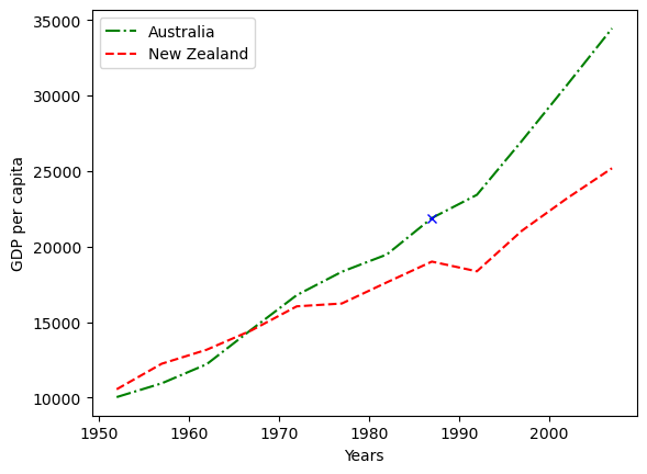
Australia	10039.59564	10949.64959	12217.22686	14526.12465	16788.62948	18334.19751	19477.00928	21888.88903	23424.76683	26997.93657	30687.75473	34435.36744
New Zealand	10556.57566	12247.39532	13175.67800	14463.91893	16046.03728	16233.71770	17632.41040	19007.19129	18363.32494	21050.41377	23189.80135	25185.00911

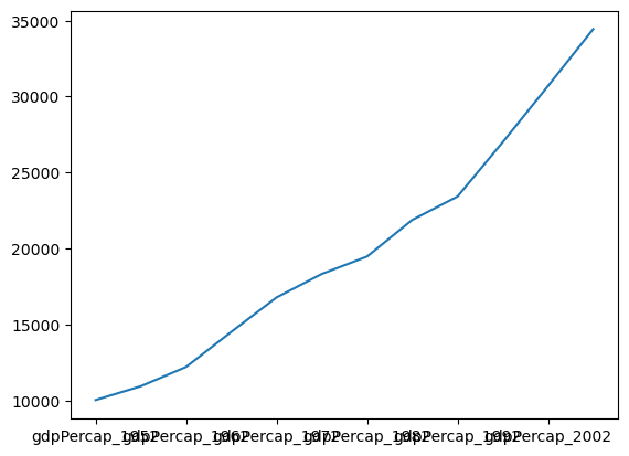
data_o.loc["Australia"].plot()

<Axes: >

#data_o.columns
#Converting Column names into Integers
years = data_o.columns.str.strip('gdpPercap_').astype(int)
years

Index([1952, 1957, 1962, 1967, 1972, 1977, 1982, 1987, 1992, 1997, 2002, 2007], dtype='int32')

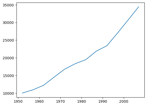
#Renaming column names
data_o.columns = years
data_o

	1952	1957	1962	1967	1972	1977	1982	1987	1992	1997	2002	2007
country
Australia	10039.59564	10949.64959	12217.22686	14526.12465	16788.62948	18334.19751	19477.00928	21888.88903	23424.76683	26997.93657	30687.75473	34435.36744
New Zealand	10556.57566	12247.39532	13175.67800	14463.91893	16046.03728	16233.71770	17632.41040	19007.19129	18363.32494	21050.41377	23189.80135	25185.00911

data_o.loc["Australia"].plot()

<Axes: >

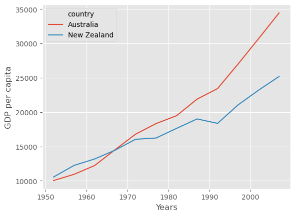
#Changing style of plot
plt.style.use('ggplot')
data_o.T.plot()
plt.ylabel('GDP per capita')
plt.xlabel('Years')

Text(0.5, 0, 'Years')

#Another way of plotting
gdp_nz = data_o.loc["New Zealand"]
gdp_aus = data_o.loc["Australia"]
data_o[1987]

country
Australia      21888.88903
New Zealand    19007.19129
Name: 1987, dtype: float64

plt.style.use('default')
plt.plot(years,gdp_aus,"g-.", label="Australia")
plt.plot(years,gdp_nz,"r--", label="New Zealand")
##Plotting one specific point
plt.plot(1987,data_o.loc["Australia",1987],"bx")
#Axis labels
plt.ylabel('GDP per capita')
plt.xlabel('Years')
#adding legend
plt.legend(loc="best")
#plt.xticks(rotation=60)
plt.savefig("oceania.png")

Other Types of plots: Bar and Scatter Plots

#Creating example Data
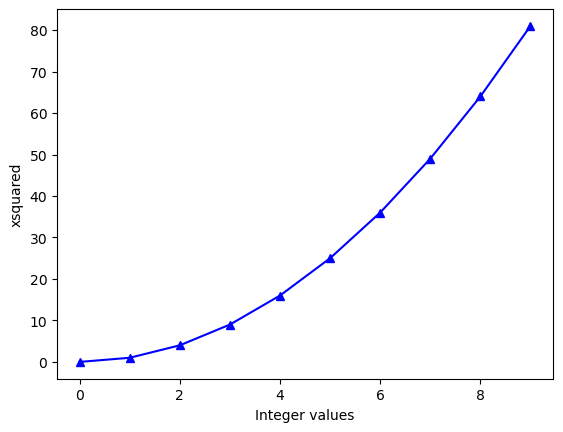
x = np.arange(10)
y = x**2
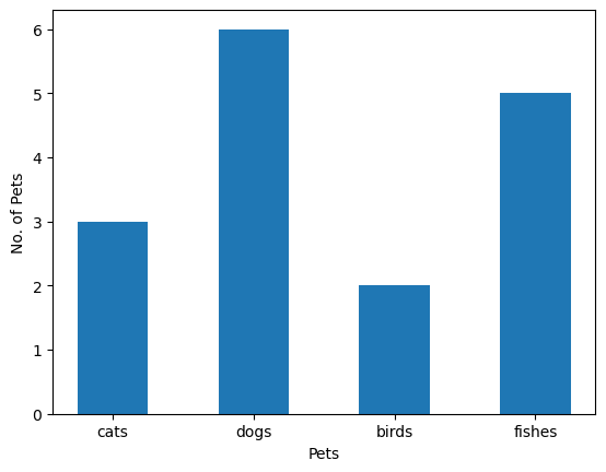
b1 = ["cats", "dogs", "birds", "fishes"]
b2 = [3,6,2,5]
#s1 = np.arange(10)
s = np.random.randint(2,9,10)
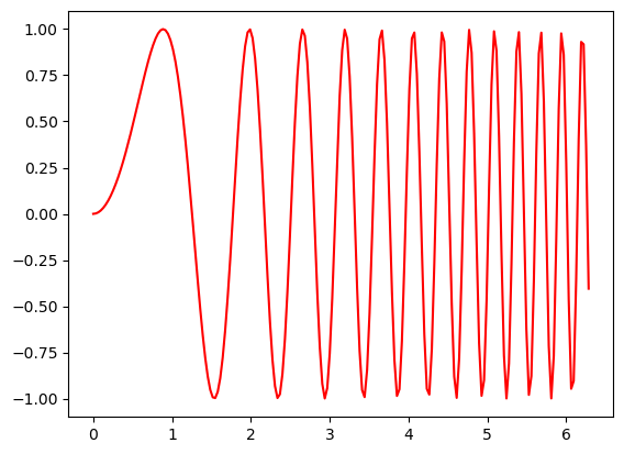
x1 = np.linspace(0, 2*np.pi, 200)
y1 = np.sin(2*(x1**2))

#line plot
plt.plot(x,y, 'b^-')
plt.xlabel("Integer values")
plt.ylabel("xsquared")

Text(0, 0.5, 'xsquared')

#Line plot 2
plt.plot(x1,y1, 'r')

[<matplotlib.lines.Line2D at 0x2367b074f90>]

#Bar plots
plt.bar(b1,b2,width=0.5)
plt.xlabel("Pets")
plt.ylabel("No. of Pets")

Text(0, 0.5, 'No. of Pets')

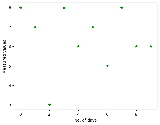
#Scatter plots
plt.scatter(x,s, c = "green", marker = "*")
plt.xlabel("No. of days")
plt.ylabel("Measured Values")

Text(0, 0.5, 'Measured Values')

Subplots

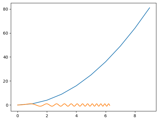
fig, ax = plt.subplots()
#print(ax)
ax.plot(x,y)
ax.plot(x1,y1)

[<matplotlib.lines.Line2D at 0x2367b0ab750>]

fig, ax = plt.subplots(2)
#print(ax)
ax[1].plot(x,y, "b^-")
ax[0].plot(x1,y1, 'r')

[<matplotlib.lines.Line2D at 0x2367b0e8f50>]

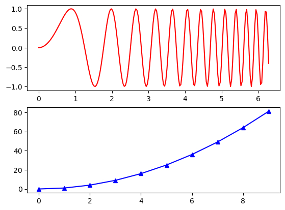
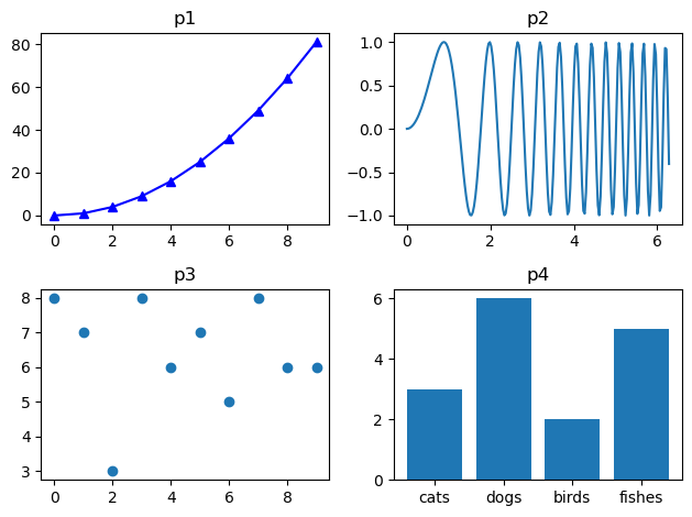
fig1, ax1 = plt.subplots(2,2)
#print(fig1, ax1)
ax1[0,0].plot(x,y,"b^-")
ax1[0,0].set_title("p1")
ax1[0,1].plot(x1,y1)
ax1[0,1].set_title("p2")
ax1[1,0].scatter(x,s)
ax1[1,0].set_title("p3")
ax1[1,1].bar(b1,b2)
ax1[1,1].set_title("p4")
fig1.tight_layout()

Other types of plots

reference: http://www.math.buffalo.edu/~badzioch/MTH337/PT/PT-image_processing/PT-image_processing.html

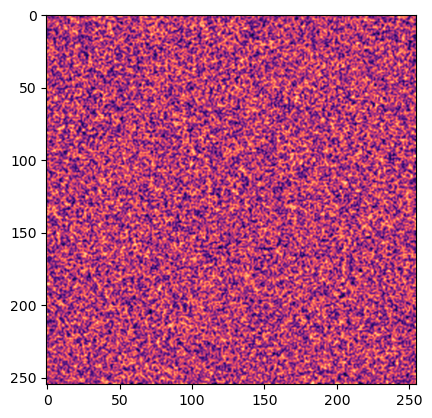
np.random.seed(2023)
mat2 = np.random.randint(-255,255,65025).reshape(255,255)
#plt.imshow(mat2)
#plt.imshow(mat2, interpolation = "bicubic") ## bilinear, gaussian, lanczos, bicubic
plt.imshow(mat2, interpolation = "bicubic", cmap = 'magma') #cmaps: viridis, plasma, inferno, magma
#plt.colorbar() ##Add colorbar for to show values

<matplotlib.image.AxesImage at 0x2367c345410>

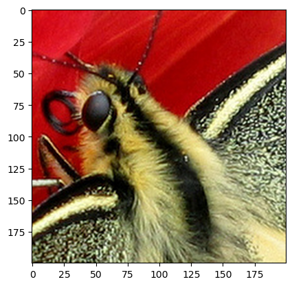
#!wget https://upload.wikimedia.org/wikipedia/commons/3/3d/Fesoj_-_Papilio_machaon_%28by%29.jpg -O butterfly.JPG

butterfly = plt.imread("butterfly.jpg")
#print(type(butterfly))
#plt.imshow(butterfly)
plt.imshow(butterfly[200:400,350:550], interpolation="lanczos")

<matplotlib.image.AxesImage at 0x2367c3a5410>

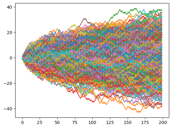
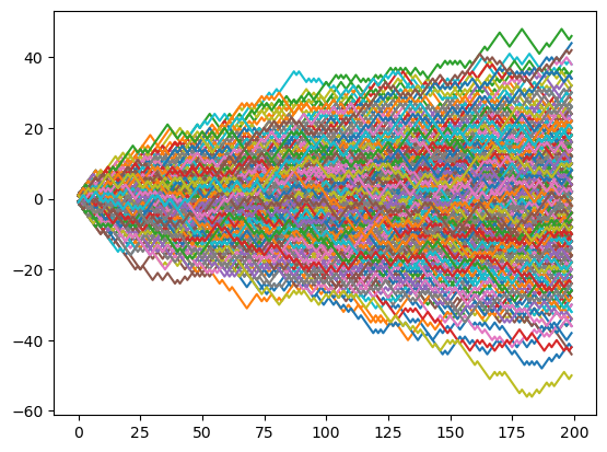
Example: Random Walk

Solution 1

def random_walk(num_steps):
    walk = np.zeros(num_steps)
    for step in range(len(walk)):
        #Coin flip result
        coin_flip_result = np.random.randint(2)
        if coin_flip_result == 0:
            #Heads
            walk[step] = walk[step-1]+1
        else:
            #Tails
            walk[step] = walk[step-1]-1
    plt.plot(walk)

%%time
walk_range = 1000
num_steps = 200
for walk in range(walk_range):
    random_walk(num_steps)

CPU times: total: 688 ms
Wall time: 697 ms

Solution 2

%%time
for walk in range(walk_range):
    plt.plot(np.cumsum([1 if i else -1 for i in np.random.randint(2, size=num_steps)]))

CPU times: total: 297 ms
Wall time: 306 ms