Nearest Neighbours Classification#
teaching: 20 exercises: 0 questions:
“How to use K-Nearest Neighbour in Machine Learning model” objectives:
“Learn how to use KNN in ML model” keypoints:
“KNN”
K-Nearest Neighbour#
Nearest-neighbour classification is very simple and intuitive. Consider a two-dimensional graphical representation of our data:
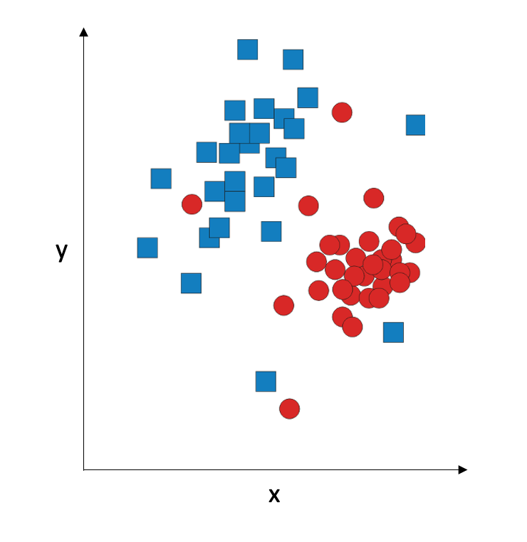
The idea is: given a point (an observation), we assign it to the same class as its nearest neighbour. So there is no training, and in the testing phase, we compute the Euclidean distances to all training data points and assign the observation to the same class as the training data point which is the closest. So it is really fast, but it only works on data where classes form very tight clusters:

If the clusters are less tight, the performance suffers; if the classes overlap, the performance gets really bad. This method is extremely sensitive to outliers and to noisy data.
It is possible to stabilize it, by considering not just the nearest neighbour, but a set of nearest neighbours. We can assign it to the class that gets the majority votes of 3 nearest neighbours, or 6 nearest neighbours. The number of nearest neighbours to be used is denoted with K; choise of K might impact our classification:

So, what is the best K? There is no general answer because it depends on the data. K is called the hyperparameter of the classifier: it is a parameter of the model has to be specified externally.
There is, however, a way to estimate K during our training. Remember that we used to split our data into training set and test set. Alternatively, we can split it into three subsets: traiing set, test set, and validation set. Using different values of K, we classify the observations in the validation set, and figure out which K gives the best performance. Then, we apply this value when we predict the test set.
Here’s the R implementation:
library(caret)
data(iris)
set.seed(123)
indT <- createDataPartition(y=iris$Species,p=0.6,list=FALSE)
training <- iris[indT,]
testing  <- iris[-indT,]

ModFit_KNN <- train(Species~.,training,method="knn",tuneGrid = expand.grid(k = 1:25))

ggplot(ModFit_KNN$results,aes(k,Accuracy))+
  geom_point(color="blue")+
  labs(title=paste("Optimum K is ",ModFit_KNN$bestTune),
       y="Accuracy")

predict_KNN<- predict(ModFit_KNN,newdata=testing)
confusionMatrix(testing$Species,predict_KNN)
Here, we go from K=1 to K=25. The Caret train function takes care of creating the validation set and applying these value of K to classify it.
The process of determining the optimal value of the hyperparameter is called hyperparameter optimization, and it is very useful. For example, in SVM the hyperparameter is the cost of errors; we can loop through different settings of cose to determine the best one. However, this might take a long time. Luckily, this process is highly parallelizable, so the Palmetto cluster is a good place to do it.