Classification with decision boundaries

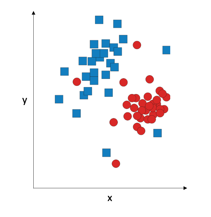
Let’s discuss the problem of multivariate classification. “Multivariate” means that we have more than one input variable, and we will consider the interaction between the input variables when we classify them. For simplicity, we assume we have two input variables, x and y. For this two-dimensional case, we can plot the data graphically. Let’s say we have two classes; we will represent them with blue squares and red circles.

Many classifiers attempt to solve the classification problem by coming up with the decision boundary: the line (straight or curved) that separates the two classes from each other. This separation does not have to be perfect; in fact, if you try to have a perfect separation using a complex curve, you might end up with overfitting:

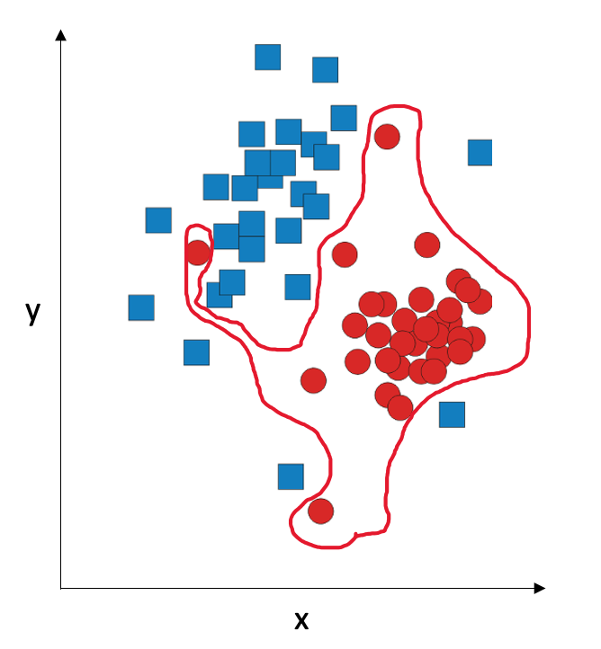
A more robust strategy is to be OK that we won’t have 100% accuracy on the training set, and try to create a decision boundary which is a straight line or a low-degree polynomial.

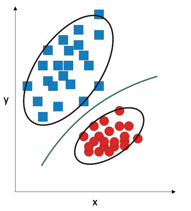
Historically, the first classifier was designed by Ronald Fisher in 1936; it is now called Fisher’s Linear Discriminant, or simply Linear Discriminant. He made the assumption that the two classes are both sampled from two-dimensional Gaussian distribution:

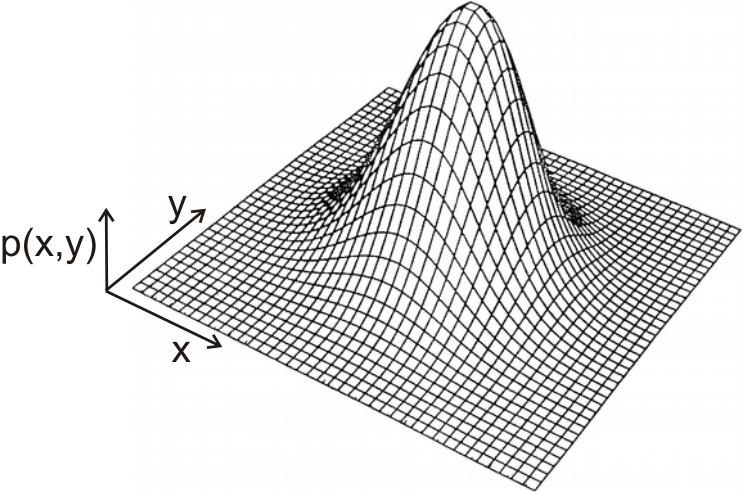
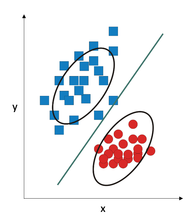
A Gaussian distribution is a cloud that is centered at the mean. It has two parameters: the mean (the location of the center of the cloud) and the covariance matrix (which defines the shape of the cloud). Linear Discriminant assumes that the two classes come from two Gaussian distributions, with different means but with the same covariance matrix. Mathematically, the decision boundary in this situation is a straight line: points that fall on one or the other side of the straight line have a higher probability of belonging to one or the other class, and points that fall exactly on that straight line have the same probability of belonging to the first and the second class.

Linear discriminant analysis works well in small samples, as long as number of variables is less than the number of observations. It is also fast and robust. However, it underperforms if the underlying assumption is not true, that is, if the covariance of the variables is very different in two classes (for example, if the “cloud” is denser in one class and sparser in the other class). In this situation, we can adjust our assumption: we can assume that the two classes come from two Gaussian distributions with different means and different covariance matrices. In this situation, the decision boundary becomes a second-degree polynomial function:

Quadratic discriminant is a very versatile classifier which works well in situations where the linear discriminant breaks down. However, it has roughly twice as much parameters that need to be estimated, so it needs larger amounts of training data.

A third classifier that uses decision boundaries is Support Vector Machines (SVM). It works very differently: it does not have any assumptions about the distribution of the data. It tries to draw a straight line between the two classes so their separation is maximal. For this purpose, it finds a subset of points in each class that lie closest to the other class, and uses these points to draw the separation margin:

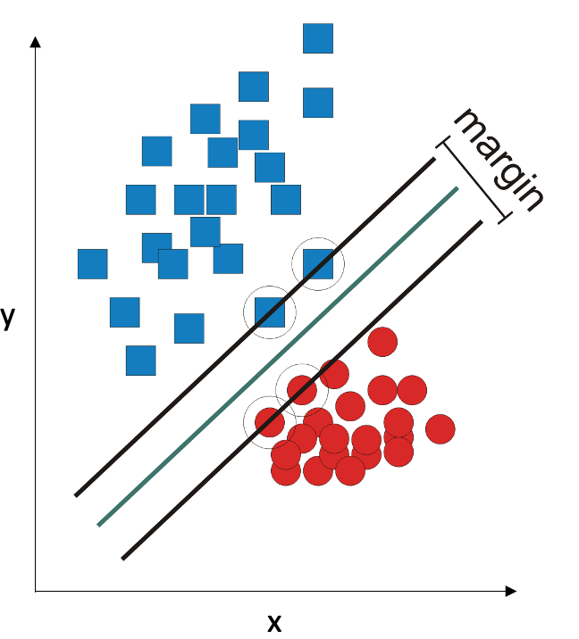
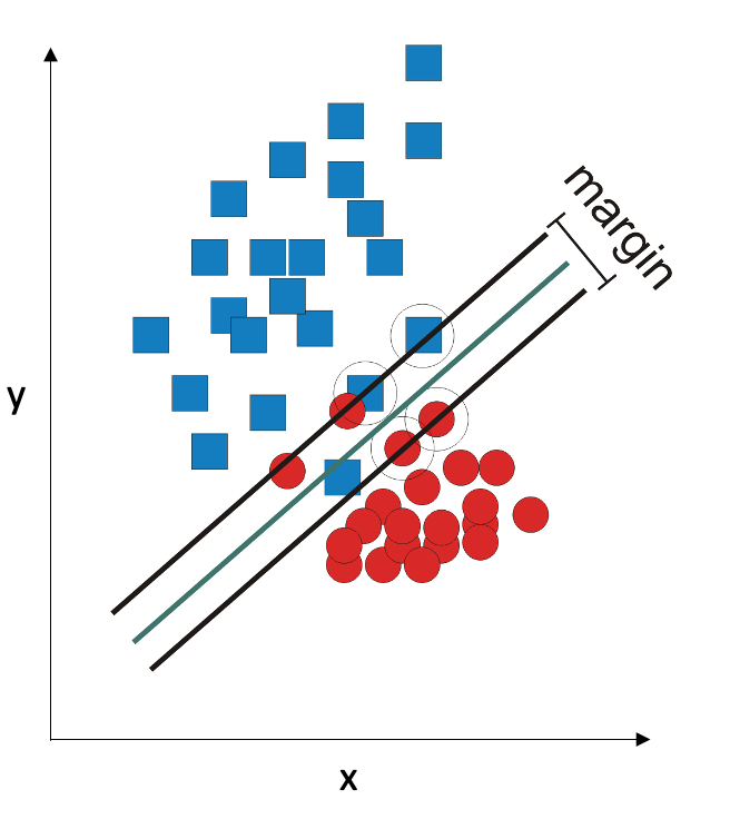
In this example, it is indeed possible to draw a straight line that separates the two classes. If it is impossible, the SVM algorithm gives itself permission to make some errors: it tries to draw the line so the errors are not greater than some threshold.

SVM is a very robust classifier: it works well in small samples and in situations where the number of observations is less than the number of variables. It can also use decision boundaries that are not straight lines. However, it is not very practical on large data sets because it becomes very slow. Also, when doing SVM, keep in mind that it is sensitive to scale of the data, so it’s usually a good idea to scale all variables to (0,1) range.

In Caret, these three classifiers can be performed with the train function. For linear discriminant, you need to set method='lda'; for quadratic discriminant, method='qda'. For SVM with linear (straight line) decision boundary, you set method = 'svmLinear' (you can also specify cost, which is the amount of error you are willing to tolerate). For non-linear boundaries, you can set method to 'svmPoly', 'svmRadial', etc. – see the list of methods supported by Caret. I used two classes in my examples, but all these methods work with any number of classes.

If the number of observations is less than the number of variables, linear and quadratic discriminants won’t work. The way around it is to use principal component analysis (PCA), where we approximate the data with a small orthogonal set of new variables(principal components), each capturing an important trend in the data. This way, if several variables are correlated, they end up in the same principal component. Essentially, our data are approximated ith a small set of principal components; this approximaition is then fed into linear or quadratic discriminants. This method is very robust to noise.