Regression and Classification with Fully Connected Neural Networks

Regression and Classification with Fully Connected Neural Networks#

Deep learning is a large, developing field with many sub-communities, a constant stream of new developments, and unlimited application areas. Despite this complexity, most deep learning techniques share a relatively small set of algorithmic building blocks. The purpose of this notebook is to gain familiarity with some of these core concepts. Much of the intuition you develop here is applicable to the neural networks making headline news from the likes of OpenAI. To focus this notebook, we will consider the two main types of supervised machine learning:

Regression: estimation of continuous quantities
Classification: estimation of categories or discrete quantities

We will create “deep learning” models for regression and classification. We will see the power of neural networks as well as the pitfalls.

# libraries we will need
import torch
from torch import nn
import numpy as np
from torch.distributions import bernoulli
import matplotlib.pyplot as plt

# set random seeds for reproducibility
torch.manual_seed(42)
np.random.seed(42)

Tasks to solve in this notebook#

Regression#

torch.randn?

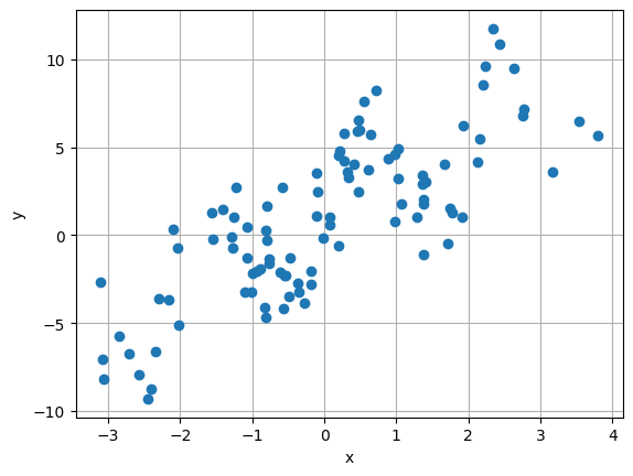
# make some fake regression data
n_samples_reg = 100
x_reg = 1.5 * torch.randn(n_samples_reg, 1)
y_reg = 2 * x_reg + 3.0*torch.sin(3*x_reg) + 1 + 2 * torch.randn(n_samples_reg, 1)
y_reg = y_reg.squeeze()

plt.plot(x_reg, y_reg, 'o')
plt.xlabel('x')
plt.ylabel('y')
plt.grid()

Classification#

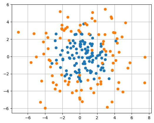
# fake classification data
n_samples_clf = 200
x_clf = 2.5*torch.randn(n_samples_clf, 2)
d = torch.sqrt( x_clf[:, 0]**2 +  x_clf[:, 1]**2 )
y_clf = d<torch.pi

# swap some labels near the boundary
width = 0.7
pgivd = 0.3 * width**2 / ((d - torch.pi)**2 + width**2)
swaps = bernoulli.Bernoulli(pgivd).sample().type(torch.bool)
y_clf[swaps] = ~y_clf[swaps]

plt.plot(x_clf[y_clf, 0], x_clf[y_clf,1], 'o', label='positive')
plt.plot(x_clf[~y_clf, 0], x_clf[~y_clf,1], 'o', label='negative')
plt.gca().set_aspect(1)
plt.grid()

The Simplest “Deep Learning” Model: Linear Regression#

Initializing our model#

Good old fashioned linear model: $y = wx + b$.

# Pytorch's `nn` module has lots of neural network building blocks
# nn.Linear is what we need for y=wx+b
reg_model = nn.Linear(in_features = 1, out_features = 1)

Question

What do you think the arguments `in_features` and `out_features` mean? When might they not be 1?

# pytorch randomly initializes the w and b
reg_model.weight, reg_model.bias

# let's look at some predictions
with torch.no_grad():
    y_reg_init = reg_model(x_reg)
    
y_reg_init[:5]

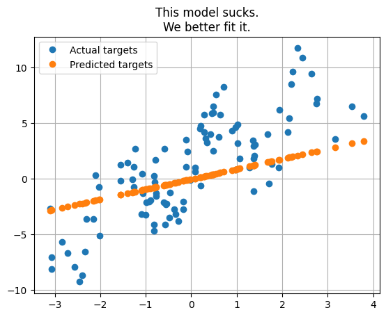
# plot the predictions before training the model
plt.plot(x_reg, y_reg, 'o', label='Actual targets')
plt.plot(x_reg, y_reg_init, 'o', label='Predicted targets')
plt.grid()
plt.legend()
_ = plt.title("This model sucks.\nWe better fit it.")

Anatomy of a training loop#

Basic idea:

Start with random parameter values
Define a loss/cost/objective measure to optimize
Use training data to evaluate the loss
Update the model to reduce the loss (use gradient descent)
Repeat until converged

Basic weight update formula: $ w_{i+1} = w_i - \mathrm{lr}\times \left.\frac{\partial L}{\partial w}\right|_{w=w_i} $

Question

Why the minus sign in front of the second term?

# re-initialize our model each time we run this cell
# otherwise the model picks up from where it left off
reg_model = nn.Linear(in_features = 1, out_features = 1)

# the torch `optim` module helps us fit models
import torch.optim as optim

# create our optimizer object and tell it about the parameters in our model
# the optimizer will be responsible for updating these parameters during training
optimizer = optim.SGD(reg_model.parameters(), lr=0.01)

# how many times to update the model based on the available data
num_epochs = 100

# setting up a colormap for ordered colors
import matplotlib.pyplot as plt
import numpy as np

colors = plt.cm.Greens(np.linspace(0.3, 1, num_epochs // 20))

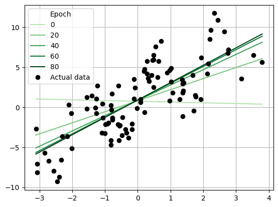
for i in range(num_epochs):
    # make sure gradients are set to zero on all parameters
    # by default, gradients accumulate
    optimizer.zero_grad()
    
    # "forward pass"
    y_hat = reg_model(x_reg).squeeze()
    
    # measure the loss
    # this is the mean squared error
    loss = torch.mean((y_hat - y_reg)**2)
    # can use pytorch built-in: https://pytorch.org/docs/stable/generated/torch.nn.functional.mse_loss.html
    
    # "backward pass"
    # that is, compute gradient of loss wrt all parameters
    loss.backward()
    
    # parameter updates
    # use the basic weight update formula given above (with slight modifications)
    optimizer.step()
    
    if i % 20 == 0:
        print(f"Epoch {i+1}. MSE Loss = {loss:0.3f}")
        with torch.no_grad():
            y_reg_init = reg_model(x_reg)
        
        ix = x_reg.argsort(axis=0).squeeze()
        plt.plot(x_reg.squeeze()[ix], y_reg_init.squeeze()[ix], '-', color=colors[i // 20], label=i, alpha=1)


plt.plot(x_reg, y_reg, 'ok', label="Actual data")
plt.grid()
_ = plt.legend(title='Epoch')

import torch
import torch.nn as nn
import torch.optim as optim
import numpy as np
import matplotlib.pyplot as plt
from matplotlib.animation import FuncAnimation
from IPython.display import HTML

# re-initialize our model each time we run this cell
# otherwise the model picks up from where it left off
reg_model = nn.Linear(in_features=1, out_features=1)

# create our optimizer object and tell it about the parameters in our model
# the optimizer will be responsible for updating these parameters during training
optimizer = optim.SGD(reg_model.parameters(), lr=0.01)

# how many times to update the model based on the available data
num_epochs = 100

# setup the figure for animation
fig, ax = plt.subplots()

# plot the initial data points
ax.plot(x_reg, y_reg, 'ok', label="Actual data")
line, = ax.plot([], [], 'g-', label="Regression Line")
epoch_text = ax.text(0.02, 0.95, '', transform=ax.transAxes)
plt.grid()
plt.legend()

# function to initialize the animation
def init():
    line.set_data([], [])
    epoch_text.set_text('')
    return line, epoch_text

# function to update the plot during each frame of the animation
def update(epoch):
    # make sure gradients are set to zero on all parameters
    # by default, gradients accumulate
    optimizer.zero_grad()
    
    # "forward pass"
    y_hat = reg_model(x_reg).squeeze()
    
    # measure the loss
    # this is the mean squared error
    loss = torch.mean((y_hat - y_reg)**2)
    
    # "backward pass"
    # that is, compute gradient of loss wrt all parameters
    loss.backward()
    
    # parameter updates
    optimizer.step()

    if epoch % 20 == 0:
        print(f"Epoch {epoch+1}. MSE Loss = {loss:0.3f}")
    
    # update the regression line
    with torch.no_grad():
        y_reg_init = reg_model(x_reg)
        ix = x_reg.argsort(axis=0).squeeze()
        line.set_data(x_reg.squeeze()[ix], y_reg_init.squeeze()[ix])
    
    # update the epoch text
    epoch_text.set_text(f'Epoch: {epoch+1}')
    
    return line, epoch_text

# create the animation
ani = FuncAnimation(fig, update, frames=num_epochs, init_func=init, blit=True)

# display the animation in Jupyter
plt.close(fig)  # prevent static image from displaying
HTML(ani.to_jshtml())

Question

What shortcomings does this model have?

🔥 IMPORTANT CONCEPT 🔥

Model bias is a type of error that occurs when your model doesn't have enough flexibility to represent the real-world data!

Linear classification#

A slight modification to the model#

We need to modify our model because the outputs are true/false

y_clf.unique()

While training the model, we cannot simply threshold the model outputs (e.g. call outputs greater than 0 ‘True’). Instead, we can have our model output a continuous number between 0 and 1. Use sigmoid to transform the output of a linear model to the range (0,1): $$ p(y=1 | \vec{x}) = \mathrm{sigmoid}(\vec w \cdot \vec x + b) $$

Question

Why doesn't thresholding work while training?

🔥 IMPORTANT CONCEPT 🔥

In order to use gradient descent, neural networks must be differentiable.

# what is sigmoid?
x_plt = torch.linspace(-10,10, 100)
y_plt = torch.sigmoid(x_plt)
plt.axvline(0, color='gray')
plt.plot(x_plt, y_plt)
plt.grid()
plt.xlabel('input')
plt.ylabel('output')
plt.gcf().set_size_inches(5,2.5)
_ = plt.title('Sigmoid Function')

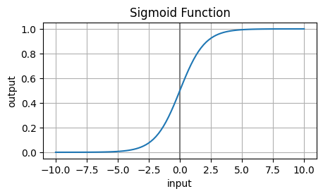
The sigmoid function is defined as:

\[\sigma(t) = \frac{1}{1 + e^{-t}}\]

# proposed new model for classification
# use nn.Sequential to string operations together
model_clf = nn.Sequential(
    nn.Linear(2, 1), # notice: we now have two inputs
    nn.Sigmoid()  # sigmoid squishes real numbers into (0, 1)
)

# what do the outputs look like?
with torch.no_grad():
    print(model_clf(x_clf)[:10])
# notice how they all lie between 0 and 1
    
# we loosely interpret these numbers as
# "the probability that y=1 given the provided value of x"

# turning probabilities into "decisions"
# apply a threshold
with torch.no_grad():
    print(model_clf(x_clf)[:10] > 0.5)

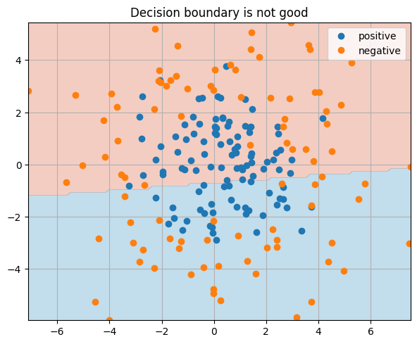
# let's see how this model does before any training

# Code to plot the decision regions
xx, yy = mg = torch.meshgrid(
    torch.linspace(x_clf[:,0].min(), x_clf[:,0].max(), 100),
    torch.linspace(x_clf[:,1].min(), x_clf[:,1].max(), 100)
)
grid_pts = torch.vstack([xx.ravel(), yy.ravel()]).T

with torch.no_grad():
    # use a 0.5 decision threshold
    grid_preds = model_clf(grid_pts).squeeze()>0.5

grid_preds = grid_preds.reshape(xx.shape)

plt.gcf().set_size_inches(7,7)
plt.plot(x_clf[y_clf, 0], x_clf[y_clf,1], 'o', label='positive')
plt.plot(x_clf[~y_clf, 0], x_clf[~y_clf,1], 'o', label='negative')
plt.gca().set_aspect(1)
plt.grid()
plt.contourf(xx, yy, grid_preds, cmap=plt.cm.RdBu, alpha=0.4)
plt.legend()
_ = plt.title("Decision boundary is not good")

Training loop#

The main difference between regression and classification is the loss function. For regression, we used mean squared error. For classification, we will use cross-entropy loss. This loss formula encourages the model to output low values for $p(y=1|x)$ when the class is 0 and high values when the class is 1.

# re-initialize our model each time we run this cell
# otherwise the model picks up from where it left off
model_clf = nn.Sequential(
    nn.Linear(2, 1),
    nn.Sigmoid()
)

# create our optimizer object and tell it about the parameters in our model
optimizer = optim.SGD(model_clf.parameters(), lr=0.01)

# torch needs the class labels to be zeros and ones, not False/True
y_clf_int = y_clf.type(torch.int16)

# how many times to update the model based on the available data
num_epochs = 1000
for i in range(num_epochs):
    optimizer.zero_grad()
    
    y_hat = model_clf(x_clf).squeeze()
    
    # measure the goodness of fit
    # need to use a different loss function here
    # this is the "cross entropy loss"
    loss = -y_clf_int * torch.log(y_hat) - (1-y_clf_int)*torch.log(1-y_hat)
    loss = loss.mean()
    # pytorch built-in: https://pytorch.org/docs/stable/generated/torch.nn.functional.binary_cross_entropy.html
    
    # update the model
    loss.backward() # gradient computation
    optimizer.step()  # weight updates
    
    if i % 100 == 0:
        print(f"Epoch {i+1}. CE Loss = {loss:0.3f}")

with torch.no_grad():
    # use a 0.5 decision threshold
    grid_preds = model_clf(grid_pts).squeeze()>0.5

grid_preds = grid_preds.reshape(xx.shape)

plt.gcf().set_size_inches(7,7)
plt.plot(x_clf[y_clf, 0], x_clf[y_clf,1], 'o', label='positive')
plt.plot(x_clf[~y_clf, 0], x_clf[~y_clf,1], 'o', label='negative')
plt.gca().set_aspect(1)
plt.grid()
plt.contourf(xx, yy, grid_preds, cmap=plt.cm.RdBu, alpha=0.4)
plt.legend()
_ = plt.title("Decision boundary is still not good")

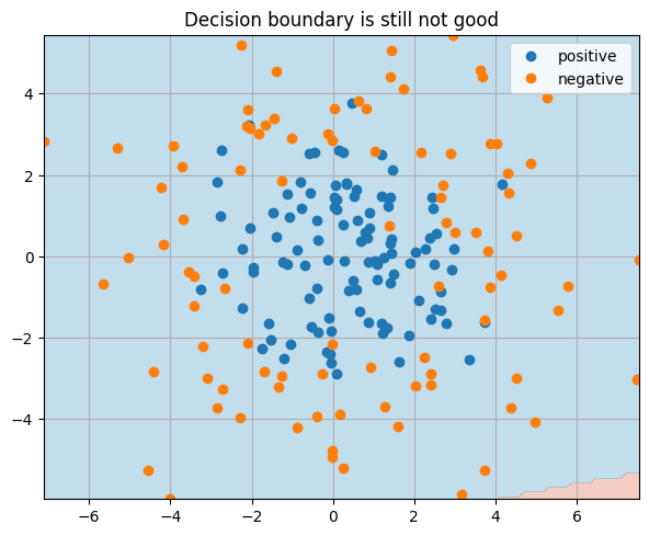
Question

Why did this experiment fail? Any ideas what we could do to make it work?

Summing up linear models#

Sometimes linear models can be a good approximation to our data. Sometimes not.

Linear models tend to be biased in the statistical sense of the word. That is, they enforce linearity in the form of linear regression lines or linear decision boundaries. The linear model will fail to the degree that the real-world data is non-linear.

Getting non-linear with fully-connected neural networks#

We can compose simple math operations together to represent very complex functions.

A few helper functions#

def train_and_test_regression_model(model, num_epochs=1000, reporting_interval=100):

    # create our optimizer object and tell it about the parameters in our model
    optimizer = optim.SGD(model.parameters(), lr=0.01)

    # how many times to update the model based on the available data
    for i in range(num_epochs):
        optimizer.zero_grad()

        y_hat = model(x_reg).squeeze()

        # measure the goodness of fit
        loss = torch.mean((y_hat - y_reg)**2)

        # update the model
        loss.backward() # gradient computation
        optimizer.step()  # weight updates

        if i % reporting_interval == 0:
            print(f"Epoch {i+1}. MSE Loss = {loss:0.3f}")
            
    with torch.no_grad():
        y_reg_init = model(x_reg)
    plt.plot(x_reg.cpu(), y_reg.cpu(), 'o', label='Actual targets')
    plt.plot(x_reg.cpu(), y_reg_init.cpu(), 'x', label='Predicted targets')
    plt.grid()
    plt.legend()

def train_and_test_classification_model(model, num_epochs=1000, reporting_interval=100):

    # create our optimizer object and tell it about the parameters in our model
    optimizer = optim.SGD(model.parameters(), lr=0.01)

    # how many times to update the model based on the available data
    for i in range(num_epochs):
        optimizer.zero_grad()

        y_hat = model(x_clf).squeeze()

        # measure the goodness of fit
        # need to use a different loss function here
        loss = -y_clf_int * torch.log(y_hat) - (1-y_clf_int)*torch.log(1-y_hat)
        loss = loss.mean()

        # update the model
        loss.backward() # gradient computation
        optimizer.step()  # weight updates
    
        if i % reporting_interval == 0:
            print(f"Epoch {i+1}. CE Loss = {loss:0.3f}")   
            
    with torch.no_grad():
        grid_preds = model(grid_pts).squeeze()>0.5

    grid_preds = grid_preds.reshape(xx.shape)

    plt.gcf().set_size_inches(7,7)
    plt.plot(x_clf[y_clf, 0], x_clf[y_clf,1], 'o', label='positive')
    plt.plot(x_clf[~y_clf, 0], x_clf[~y_clf,1], 'o', label='negative')
    plt.gca().set_aspect(1)
    plt.grid()
    plt.contourf(xx, yy, grid_preds, cmap=plt.cm.RdBu, alpha=0.4)
    plt.legend()

Regression#

What about nested linear models? Might this do something interesting? $$ y = w_1(w_0 x + b_0) + b_1 $$

# We can build more complex models by stringing together more operations inside nn.Sequential:
model =  nn.Sequential(
    nn.Linear(in_features = 1, out_features = 1),
    nn.Linear(1,1)
)

train_and_test_regression_model(model)
_ = plt.title("But wait, that's still just a line?!")

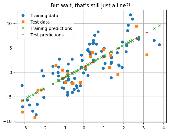
Question

Why is it still just a line? How can we fix it?

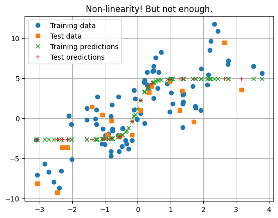
# We need a non-linearity between the two linear operations
model =  nn.Sequential(
    nn.Linear(in_features = 1, out_features = 1),
    nn.Tanh(),
    nn.Linear(1,1)
)
# this model does not reduce to a linear operation

train_and_test_regression_model(model)
_ = plt.title("Non-linearity! But not enough.")

# Let's really crank up the number of hidden nodes
model =  nn.Sequential(
    nn.Linear(in_features = 1, out_features = 30),
    nn.Tanh(),
    nn.Linear(30,30),
    nn.Tanh(),
    nn.Linear(30,30),
    nn.Tanh(),
    nn.Linear(30,30),
    nn.Tanh(),
    nn.Linear(30,30),
    nn.Tanh(),
    nn.Linear(30,30),
    nn.Tanh(),
    nn.Linear(30,1)
)

train_and_test_regression_model(model, num_epochs=50_000, reporting_interval=5000)

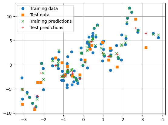
Question

What is wrong with this picture?

with torch.no_grad():
    x_grid = torch.linspace(x_reg.min(), x_reg.max(), 200)[:,None]
    y_reg_grid = model(x_grid)
    y_reg_init = model(x_reg)
plt.plot(x_reg.cpu(), y_reg.cpu(), 'o', label='Actual targets')
plt.plot(x_reg.cpu(), y_reg_init.cpu(), 'x', label='Predicted targets')
plt.plot(x_grid.cpu(), y_reg_grid.cpu(), 'k-', label='Predicted')
plt.grid()
plt.legend()

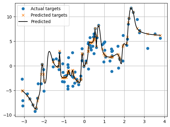
Question

Where is overfitting most severe? How might having more data alleviate the problem?

🔥 IMPORTANT CONCEPT 🔥

Overfitting is a type of error that occurs when your model memorizes the training samples and fails to generalize to unseen data. This usually ocurrs when the model has excess capacity.

😅 EXERCISE 😅

Using the code cell below, design and test a model that gets it "just right".

#model = your model goes here

# train_and_test_regression_model(model, num_epochs=10000, reporting_interval=1000)

Classification#

Let’s apply the same non-linear treatment to the case of classification.

model =  nn.Sequential(
    nn.Linear(in_features = 2, out_features = 2),
    nn.Tanh(),
    nn.Linear(2,1),
    nn.Sigmoid()
)

train_and_test_classification_model(model, 10_000, 1000)
_ = plt.title("Not non-linear enough")

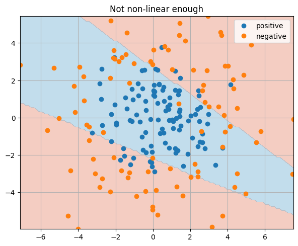
Question

What would overfitting look like in this type of graph?

model =  nn.Sequential(
    nn.Linear(in_features = 2, out_features = 50),
    nn.Tanh(),
    nn.Linear(50,50),
    nn.Tanh(),
    nn.Linear(50,50),
    nn.Tanh(),
    nn.Linear(50,50),
    nn.Tanh(),
    nn.Linear(50,50),
    nn.Tanh(),
    nn.Linear(50,50),
    nn.Tanh(),
    nn.Linear(50,1),
    nn.Sigmoid()
)

train_and_test_classification_model(model, 30000, 3000)
_ = plt.title("What went wrong here?")

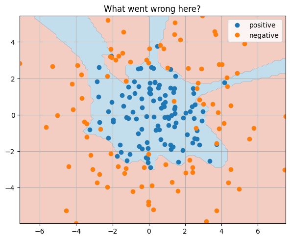
Question

What's wrong with this picture?

😅 EXERCISE 😅

Using the code cell below, design and test a model that gets it "just right".

#model = your model goes here

# train_and_test_classification_model(model, 20000, 2000)

Summing up fully connected neural networks#

Fully connected neural networks can represent highly non-linear functions
We can learn good functions through gradient descent
Overfitting is a big problem

These concepts apply to nearly any neural network trained with gradient descent from the smallest fully connected net to GPT-4.

Regression and Classification with Fully Connected Neural Networks

Contents

Regression and Classification with Fully Connected Neural Networks#

Tasks to solve in this notebook#

Regression#

Classification#

The Simplest “Deep Learning” Model: Linear Regression#

Initializing our model#

Anatomy of a training loop#

Linear classification#

A slight modification to the model#

Training loop#

Summing up linear models#

Getting non-linear with fully-connected neural networks#

A few helper functions#

Regression#

Classification#

Summing up fully connected neural networks#