Small Language Models: an introduction to autoregressive language modeling

Small Language Models: an introduction to autoregressive language modeling#

This notebook was partly inspired by this blog post on character-level bigram models: https://medium.com/@fareedkhandev/create-gpt-from-scratch-using-python-part-1-bd89ccf6206a

import os
os.environ["TOKENIZERS_PARALLELISM"] = "false"

The language modeling task#

What is language modeling?#

In this notebook, we take a first look at the language modeling task. “Language Modeling” has two parts:

“Language” is what it sounds like. For our purposes, we will always represent language with text. We will also talk about
- tokens: pieces of text. These could be words, word chunks, or individual characters.
- documents: a sequence of tokens about something. These could be individual tweets, legal contracts, love letters, emails, or journal abstracts.
- dataset: a collection of document. We will be using a PubMed dataset containing 50 thousand abstracts.
- vocabulary: the set of all unique tokens in our dataset.
“Modeling” refers to creating a mathematical structure that, in some way, corresponds to observed data. In this case, the data is language, so the model should quantiatively capture something about the nature of language. We need to make this more concrete.

Language modeling as probabilistic modeling#

Let’s try to make the idea of mathematically modeling language more concrete. We will develop models for the vector of tokens that appear in a document. We denote this as $$ p(\langle w_i\rangle_{i=1}^{L}) $$ where $w_i$ is the token at position $i$ in a document and $L$ is the number of words in the document. The angle bracket with limits notation here denotes the vector of all tokens specified by the limits.

If we knew this joint distribution, we could sample new documents $d$: $$ d \sim p(\langle w_i\rangle_{i=1}^{L}) $$ This is called _language generation_ because $d$ is not in the dataset that we used to learn $p(\langle w_i\rangle_{i=1}^{L})$, but it “looks like” it is from that dataset.

Autoregressive language modeling#

Let’s make a simplifying assumption. Let’s assume that the probability for token $i$ only depends on the previous tokens as shown in this figure (Notice: no arrows going from right to left.)

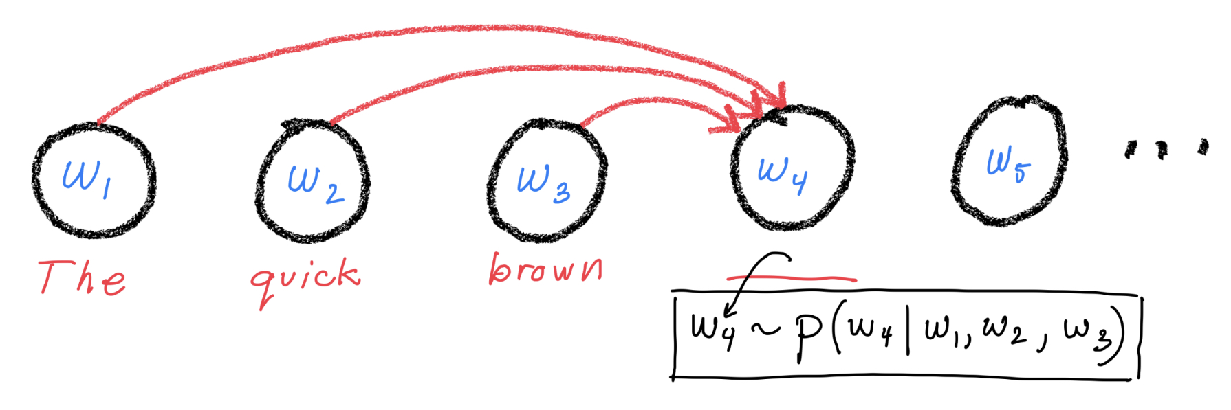
Mathematically, this can be expressed as: $$ p(w_i | \langle w_j\rangle_{j\neq i}) = p(w_i | \langle w_j\rangle_{j=1}^{i-1}) $$ This gives us a natural way to sample documents because it implies that $$ p(\langle w_i\rangle_{i=1}^{L}) = p(w_1)\prod_{j=2}^L p(w_j | \langle w_i\rangle_{i=1}^{j-1}) $$ So, to generate a new document, we can

start with a prompt token or token sequence
sample the next token conditioned on the prompt and append it to the prompt
sample the next token conditioned on the appended prompt and append it to the appended prompt
and so on….

This is how ChatGPT works! This approach goes by the names autoregressive language modeling or causal language modeling.

This is not how all language modeling works. BERT, for instance, uses masked language modeling, where random tokens in a sequence are sampled by considering the tokens at all other positions. Word2Vec models tokens using a neighborhood of nearby tokens.

Also, we still haven’t said anything about how you actually write down the functional form of $p(w_i | \langle w_j\rangle_{j=1}^{i-1})$. There are many possibly architectures (an incomplete list in approximate historical ordering):

Markov model
1D CNN
RNN
LSTM/GRU
Transformer

We will spend the next notebook digging deep into the last option. Before we do, though, let’s try to get a better understanding of language models by looking closely at a simple Markov model.

Large Small Language Model#

The simplest, non-trivial model#

Before we move on to attention, transformers, and LLMs, let’s first write down and fit a very simple language model for the PubMed dataset. This will provide a baseline for more sophisticated techniques and will give us a better understanding of how autoregressive language modeling works. Most of the lessons learned will transfer directly to the LLM case.

The simplest, non-trivial model comes from assuming that the distribution for token $i$ only depends on token $i-1$. Graphically:

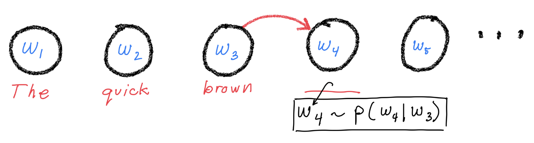
With this Markov assumption, the conditional distribution for token $i$ simplifies to $$ p(w_i | \langle w_j\rangle_{j=1}^{i-1}) = p(w_i | w_{i-1}) $$

The probability distribution for the entire sequence is then $$ p(\langle w_i\rangle_{i=1}^{L}) = p(w_{1})\prod_{i=2}^{L}p(w_{i}|{w}_{i-1}) $$ allowing us to generate sequences as described above.

In what ways might this be an inadequate model for human language?

Estimating the model from data#

How can we estimate this model mathematically?

We start by observing that the model only depends on a set of probabilities describing the liklihood of one word given another word. These probabilities are called transition matrix elements, $$ T_{\alpha\beta} = p(w_i=\alpha | w_{i-1}=\beta)\\ $$ where the matrix elements satisfy $$ T_{\alpha\beta} \geq 0 \\ \sum_\alpha T_{\alpha\beta} =1 $$ where $\alpha$ and $\beta$ are two tokens in our vocabulary. If the vocab size is $V$, the estimation task comes down to inferring the $V\times V$ transition matrix elements describing the probability of going from any word to any other word.

Estimating with frequency tables#

One straightforward way to estimate these probabilities would be to list all of the neighbor pairs of tokens in our dataset and for each conditioning token $\beta$ look at the share into each choice of $\alpha$. This can be made to work, though we would have to deal with the fact that many token pairs will never appear.

Estimating with gradient descent#

In the code below, we will take a different approach. We will estimate the probabilities using a maximum liklihood based approach with gradient descent. For the Markov model, the two approaches are formally equivalent up to how they deal with the missing pairs. However, the gradient descent approach will generalize to more complicated models including transformer-based LLMs!

Enough talk#

Load our PubMed data#

Make sure you have the dataset.py in your working directory.

wget https://raw.githubusercontent.com/clemsonciti/rcde_workshops/master/pytorch_llm/dataset.py

# use the dataset.py file
from dataset import PubMedDataset
dataset = PubMedDataset("/project/rcde/datasets/pubmed/mesh_50k/splits/")

Found cached dataset text (/home/dane2/.cache/huggingface/datasets/text/default-cadbbf8acc2e2b5a/0.0.0/cb1e9bd71a82ad27976be3b12b407850fe2837d80c22c5e03a28949843a8ace2)

dl_train = dataset.get_dataloader('train', batch_size=3)
batch = next(iter(dl_train))
print(batch.keys())

dict_keys(['input_ids', 'token_type_ids', 'attention_mask'])

next(iter(dl_train))

{'input_ids': tensor([[ 101, 1103, 2853,  ...,    0,    0,    0],
        [ 101, 3582,  131,  ..., 8131,  119,  102],
        [ 101, 3582,  131,  ...,    0,    0,    0]]), 'token_type_ids': tensor([[0, 0, 0,  ..., 0, 0, 0],
        [0, 0, 0,  ..., 0, 0, 0],
        [0, 0, 0,  ..., 0, 0, 0]]), 'attention_mask': tensor([[1, 1, 1,  ..., 0, 0, 0],
        [1, 1, 1,  ..., 1, 1, 1],
        [1, 1, 1,  ..., 0, 0, 0]])}

Build our small language model#

For the Markov model, we need to know the size of our vocabulary.

vocab_size = dataset.tokenizer.vocab_size
vocab_size

Yikes, that’s a big vocabulary! The size of the transition matrix will be vocab_size * vocab_size. Let’s estimate how much memory that would take to store:

# memory needed to store the transition matrix (in gigabytes)
vocab_size * vocab_size * 32 / 8 / 1e9

3.363072064

That’s huge, but let’s just try it anyway. Let’s write down our pytorch model. Just a little notation first:

$N$: The batch size in batch gradient descent
$L$, $L_\mathrm{batch}$: The document sequence length or the sequence length of the batch, respectively.
$V$: the size of our vocab

Without further ado, let’s write down the model:

import torch
import torch.nn.functional as F
class MarkovChain(torch.nn.Module):
    def __init__(self, vocab_size):
        super().__init__()

        # the transition matrix logits
        # nn.Embedding is just a matrix. Each input token will have a learnable
        # parameter vector with one element for each output token.
        # the transition matrix elements are computed by taking the softmax along the output dimension
        self.t_logits = torch.nn.Embedding(vocab_size, vocab_size)
        
        # let's start with the assumption that most transitions are very improbable
        # large negative logit -> low probability
        self.t_logits.weight.data -= 10.0

    def forward(self, x):
        logits = self.t_logits(x) 
        # logits.shape == (N, L_batch, V). Remember (batch size, sequence length, vocab size).

        return logits # turns out we never actually need to compute the softmax for MLE
    
    def numpars(self):
        return sum(p.numel() for p in self.parameters() if p.requires_grad)

Let’s try it on some actual data to make sure it works.

model = MarkovChain(vocab_size)
print("Trainable params (millions):", model.numpars()/1e6)
model

Trainable params (millions): 840.768016

MarkovChain(
  (t_logits): Embedding(28996, 28996)
)

y = model(batch["input_ids"])
y.shape

torch.Size([3, 463, 28996])

The output tensor has shape batch_size x sequence_length x vocab_size. We interpret these ouputs as the logits of the next word. The probability of the next word is then

p_next_words = y.softmax(dim=-1)

# check that the total probability over possible next tokens sums to 1:
p_next_words.sum(dim=-1)

tensor([[1.0000, 1.0000, 1.0000,  ..., 1.0000, 1.0000, 1.0000],
        [1.0000, 1.0000, 1.0000,  ..., 1.0000, 1.0000, 1.0000],
        [1.0000, 1.0000, 1.0000,  ..., 1.0000, 1.0000, 1.0000]],
       grad_fn=<SumBackward1>)

Generate text for untrained model#

def generate(model, idx, max_new_tokens):
        """
        Recursively generate a sequence one token at a time
        """
        # idx is (N, L) array of indices in the current context
        for _ in range(max_new_tokens):
            # get the predictions
            with torch.no_grad():
                logits = model(idx)  # [N, L, V]
            
            # trim last time step. It is prediction for token after end of sequence
            logits = logits[:, -1] # becomes (N, V)
            
            # apply softmax to get probabilities
            probs = F.softmax(logits, dim=-1) # (N, V)
            
            # sample from the distribution
            idx_next = torch.multinomial(probs, num_samples=1) # (N, 1)
            
            # append sampled index to the running sequence
            idx = torch.cat((idx, idx_next), dim=1) # (N, L+1)
            
        return idx

Let’s use our model to generate some sequences!

prompts = [
    "We compared the prevalence of", # organ-specific autoantibodies in a group of Helicobacter..."
    "We compared the prevalence of",
    "We compared the prevalence of"
]

prompt_ids = dataset.tokenizer(prompts, return_tensors='pt')['input_ids']
prompt_ids

tensor([[  101,  1195,  3402,  1103, 22760,  1104,   102],
        [  101,  1195,  3402,  1103, 22760,  1104,   102],
        [  101,  1195,  3402,  1103, 22760,  1104,   102]])

dataset.decode_batch(prompt_ids)

['[CLS] we compared the prevalence of [SEP]',
 '[CLS] we compared the prevalence of [SEP]',
 '[CLS] we compared the prevalence of [SEP]']

# trim off unwanted [SEP] tokens which act like our special end-of-sequence token.
prompt_ids = prompt_ids[:,:-1]
prompt_ids

tensor([[  101,  1195,  3402,  1103, 22760,  1104],
        [  101,  1195,  3402,  1103, 22760,  1104],
        [  101,  1195,  3402,  1103, 22760,  1104]])

# generate more ids
gen_ids = generate(model, prompt_ids, 15)
gen_ids

tensor([[  101,  1195,  3402,  1103, 22760,  1104, 24884, 17254, 26954,  1411,
         26075, 15522, 22389, 20553, 19476, 28335,  2227, 20974, 20500, 14507,
          2257],
        [  101,  1195,  3402,  1103, 22760,  1104,  2568, 21056,   355, 12811,
         12318, 14785,  5376, 11395,  6381,  2335,  4051, 16601,  7579,   609,
         13538],
        [  101,  1195,  3402,  1103, 22760,  1104,  5399, 22759,  9429, 20698,
         20509, 11237, 27838, 24444, 18389, 12594, 17810,  8110, 25186, 25466,
         24989]])

# decode into text 
dataset.decode_batch(gen_ids)

['[CLS] we compared the prevalence of Straits cracking tilting townhales robbery bubblesopping skipάntlbergrdesholder forced',
 '[CLS] we compared the prevalence ofline Calder ɔ Mohammed embassy convenient acted Zimbabwe Colin complete containing socks Hitler चcos',
 '[CLS] we compared the prevalence of Rights pharmacy graphicnking Latter Wingsests coldercel broader embarrassing elderggle artworks Horses']

Terrible! No surprise, though. We haven’t trained our model yet.

Before we can do that, we need an objective to optimize.

Loss function#

Remember, our goal is to learn good values for the transition matrix elements. We will do this by minimizing the cross entropy loss for next token prediction. This loss measures how likely the actual next tokens are under the predicted probability distribution over tokens.

It turns out, we never actually have to use the next token probabilities. This is because cross entropy only depends on log probabilities. So, rather than take exponentials of the logits, only to take the log again while computing cross entropy, we just stick with logits. Pytorch’s built-in cross entropy loss function expects this.

# remember what our batch of inputs abstracts looks like:
batch['input_ids'].shape

torch.Size([3, 463])

# cut the last prediction off because this corresponds to a token after the last token in the input sequence 
# y.shape == (N, L_batch, V)
pred_logits = y[:, :-1].permute(0,2,1)  # (N, V, L_batch) as needed for F.cross_entropy(.)

# cut the first word off the targets because we can't predict the distribution for the first word from the autoregressive model
targets = batch['input_ids'][:, 1:]

pred_logits.shape, targets.shape

(torch.Size([3, 28996, 462]), torch.Size([3, 462]))

Make sure these shapes make sense to you!

Use the built in pytorch function to compute cross entropy for each position in the sequence

from torch.nn import functional as F
# pytorch expects the intput to have shape `sequence_length x batch_size x vocab_size`
token_loss = F.cross_entropy(pred_logits, targets, reduction='none')
token_loss.shape

torch.Size([3, 462])

This is the loss for each token. But remember, some of those tokens are just padding to make the batch tensor rectangular. We shouldn’t count those.

We can use the attention_mask data structure output by our dataset to take care of this.

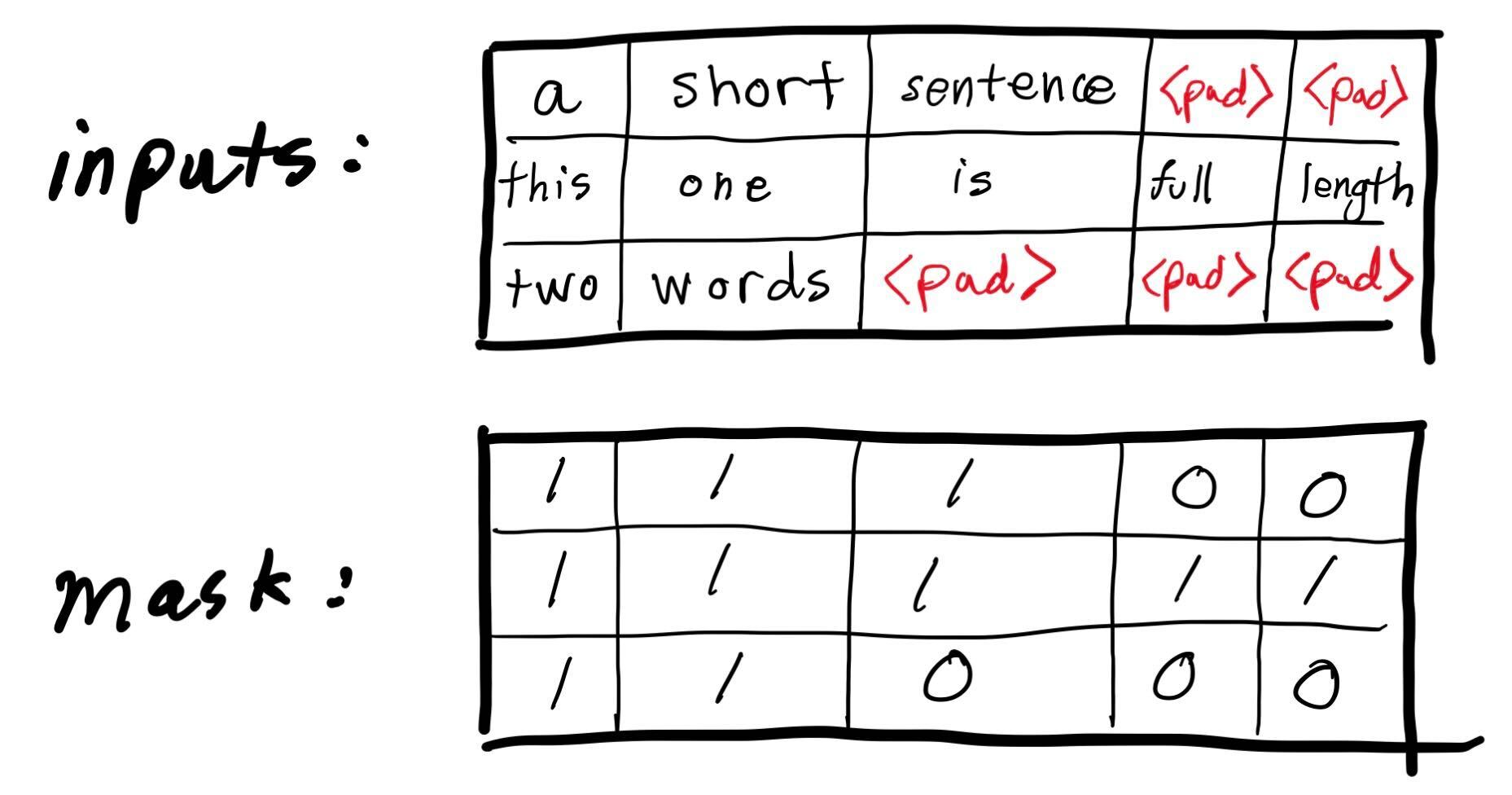
mask = batch['attention_mask'][:, 1:] # need to trim the first because our predictions are for tokens 2 through the end.
mask.shape, mask

(torch.Size([3, 462]),
 tensor([[1, 1, 1,  ..., 0, 0, 0],
         [1, 1, 1,  ..., 1, 1, 1],
         [1, 1, 1,  ..., 0, 0, 0]]))

We need to zero out the loss coming from the padding tokens and compute the average loss only counting the non-padding tokens.

Let’s put all of this logic into a function.

# let's put all this together in a custom loss function
def masked_cross_entropy(logits, targets, mask):
    """
    Args:
    - logits: The next token prediction logits. Last element removed. Shape (N, V, L-1)
    - targets: Ids of the correct next tokens. First element removed (N, L-1)
    - mask: the attention mask tensor. First element removed (N, L-1)
    """
    token_loss = F.cross_entropy(logits, targets, reduction="none")

    # total loss zeroing out the padding terms
    total_loss = (token_loss * mask).sum() 

    # average per-token loss
    num_real = mask.sum()
    mean_loss = total_loss / num_real

    return mean_loss

masked_cross_entropy(pred_logits, targets, mask)

tensor(10.7869, grad_fn=<DivBackward0>)

Time to train the model!#

This is boilerplate pytorch optimization code, so we will zip over it.

# training settings
batch_size=128
num_workers=20
num_epochs=2
learning_rate=0.1 # this model benefits from a large learning rate

# reinitialize dataset for good measure
dataset = PubMedDataset("/project/rcde/datasets/pubmed/mesh_50k/splits/")

# train/test dataloaders
dl_train = dataset.get_dataloader('train', batch_size=batch_size, num_workers=num_workers)
dl_test = dataset.get_dataloader('test', batch_size=batch_size, num_workers=num_workers)

# reinitialize the model on gpu
model = MarkovChain(vocab_size).to('cuda')

# create the pytorch optimizer
optimizer = torch.optim.AdamW(model.parameters(), lr=learning_rate)

Found cached dataset text (/home/dane2/.cache/huggingface/datasets/text/default-cadbbf8acc2e2b5a/0.0.0/cb1e9bd71a82ad27976be3b12b407850fe2837d80c22c5e03a28949843a8ace2)

# run the training loop
for epoch in range(num_epochs):
    print(f"START EPOCH {epoch+1}")
    for ix, batch in enumerate(dl_train):
        x = batch["input_ids"][:,:-1].to('cuda')  # remove last
        targets = batch["input_ids"][:,1:].to('cuda')  # remove first
        mask = batch["attention_mask"][:,1:].to('cuda') # remove first

        logits = model(x).permute(0,2,1)
        loss = masked_cross_entropy(logits, targets, mask)

        # do the gradient optimization stuff
        optimizer.zero_grad()
        loss.backward()
        optimizer.step()

        if ix % 20 ==0:
            print(f"Batch {ix} training loss: {loss.item()}")

START EPOCH 1
Batch 0 training loss: 10.774152755737305
Batch 20 training loss: 8.934335708618164
Batch 40 training loss: 7.414063930511475
Batch 60 training loss: 6.591622829437256
Batch 80 training loss: 6.113377571105957
Batch 100 training loss: 5.820305824279785
Batch 120 training loss: 5.6821465492248535
Batch 140 training loss: 5.435906410217285
Batch 160 training loss: 5.360453128814697
Batch 180 training loss: 5.330673694610596
Batch 200 training loss: 5.2893266677856445
Batch 220 training loss: 5.221299648284912
Batch 240 training loss: 5.296996593475342
Batch 260 training loss: 5.216686248779297
Batch 280 training loss: 5.102764129638672
Batch 300 training loss: 5.149473190307617
Batch 320 training loss: 5.1236572265625
Batch 340 training loss: 5.017659664154053
START EPOCH 2
Batch 0 training loss: 4.7725830078125
Batch 20 training loss: 4.893960952758789
Batch 40 training loss: 4.828927516937256
Batch 60 training loss: 4.864208698272705
Batch 80 training loss: 4.86556339263916
Batch 100 training loss: 4.830167770385742
Batch 120 training loss: 4.867104530334473
Batch 140 training loss: 4.770840167999268
Batch 160 training loss: 4.771430492401123
Batch 180 training loss: 4.816017150878906
Batch 200 training loss: 4.80755615234375
Batch 220 training loss: 4.79929256439209
Batch 240 training loss: 4.887341499328613
Batch 260 training loss: 4.846500873565674
Batch 280 training loss: 4.774038314819336
Batch 300 training loss: 4.826904773712158
Batch 320 training loss: 4.823925018310547
Batch 340 training loss: 4.747177600860596

# test; did the learning generalize?
for ix, batch in enumerate(dl_test):
    x = batch["input_ids"][:,:-1].to('cuda')  # remove last
    targets = batch["input_ids"][:,1:].to('cuda')  # remove first
    mask = batch["attention_mask"][:,1:].to('cuda') # remove first

    with torch.no_grad():
        logits = model(x).permute(0,2,1)
        loss = masked_cross_entropy(logits, targets, mask)
        
    if ix % 5 ==0:
        print(f"Batch {ix} testing loss: {loss.item()}")

Batch 0 testing loss: 4.919017314910889
Batch 5 testing loss: 4.999485969543457
Batch 10 testing loss: 5.007542610168457
Batch 15 testing loss: 4.953604698181152
Batch 20 testing loss: 4.938981533050537
Batch 25 testing loss: 5.063140869140625
Batch 30 testing loss: 4.967066287994385
Batch 35 testing loss: 4.992262840270996

The learning seems to have generalized well.

# generate some more samples now that we've trained the model
gen_samples = generate(model, prompt_ids.to('cuda'), 30)
dataset.decode_batch(gen_samples)

['[CLS] we compared the prevalence of the present study suggests an virus cystagmus Amherst Lauhul supplied Haguerid holds Prize crucial Gloucester 191ichia and imp voiced Augusta galaxy Casey dared',
 '[CLS] we compared the prevalence of feeding measurements were considered to sustainable door nodded rising Wiley multiple forms Skull draftreed Clark Mayor diagram Noctuidae myogeria Province Bellarain emeritusarean patients and',
 '[CLS] we compared the prevalence of reactive protein models of postpra Ł Т zapillous has been studied in people who were made of chronic experiments were 10 antibiotics remnant waterfront Cambodia']

The model is still terrible, though it has started to learn some very basic patterns.

Cleaning up#

We will reuse a lot this code in later sections of the workshop. I’ve pulled the import parts into utils.py. Copy the file into your working directory:

wget https://raw.githubusercontent.com/clemsonciti/rcde_workshops/master/pytorch_llm/utils.py

from utils import train, test, generate

train??

Signature: train(model, dataloader, optimizer, reporting_interval=20)
Docstring: <no docstring>
Source:   
def train(model, dataloader, optimizer, reporting_interval=20):
    model.train()
    for ix, batch in enumerate(dataloader):
        x = batch["input_ids"][:, :-1].to("cuda")  # remove last
        targets = batch["input_ids"][:, 1:].to("cuda")  # remove first
        mask = batch["attention_mask"][:, 1:].to("cuda")  # remove first

        logits = model(x).permute(0, 2, 1)
        loss = masked_cross_entropy(logits, targets, mask)

        # do the gradient optimization stuff
        optimizer.zero_grad()
        loss.backward()
        optimizer.step()

        if ix % reporting_interval == 0:
            print(f"Batch {ix} training loss: {loss.item()}")
File:      ~/Code/rcde_workshops/pytorch_llm/utils.py
Type:      function

Low rank Markov Model#

With all the setup in place, it’s easy to start experimenting with different models. We saw how huge the embedding matrix was and we worried that this would lead to bad performance. One way to get around this is to create a low-rank version of the markov model.

import torch
import torch.nn.functional as F
class MarkovChainLowRank(torch.nn.Module):
    def __init__(self, vocab_size, embed_dim):
        super().__init__()

        # We project down to size `embed_dim` then back up to `vocab_size`
        # the total number of parameters is 2 * vocab_size * embed_dim which 
        # can be much smaller than embed_dim * embed_dim
        self.t_logits = torch.nn.Sequential(
            torch.nn.Embedding(vocab_size, embed_dim),
            torch.nn.Dropout(0.1), # zero out some of the embedding vector elements randomly to prevent overfitting
            torch.nn.Linear(embed_dim, vocab_size, bias=False)
        )
        
        # let's start with the assumption that most transitions are very improbable
        # large negative logit -> low probability
        self.t_logits[-1].weight.data -= 10.0

    def forward(self, x):
        logits = self.t_logits(x) # tensor of shape (N, L, V). Remember (batch size, sequence length, vocab size).

        return logits # turns out we never actually need to compute the softmax for MLE
    
    def numpars(self):
        return sum(p.numel() for p in self.parameters() if p.requires_grad)

embedding_dim=256
learning_rate=0.001 # this model requires a more normal learning rate.
model = MarkovChainLowRank(vocab_size, embed_dim = embedding_dim)
print("Trainable params (millions):", model.numpars()/1e6)
model

Trainable params (millions): 14.845952

MarkovChainLowRank(
  (t_logits): Sequential(
    (0): Embedding(28996, 256)
    (1): Dropout(p=0.1, inplace=False)
    (2): Linear(in_features=256, out_features=28996, bias=False)
  )
)

# reinitialize dataset for good measure
dataset = PubMedDataset("/project/rcde/datasets/pubmed/mesh_50k/splits/")

# train/test dataloaders
dl_train = dataset.get_dataloader('train', batch_size=batch_size, num_workers=num_workers)
dl_test = dataset.get_dataloader('test', batch_size=batch_size, num_workers=num_workers)

# reinitialize the model on gpu
model = MarkovChainLowRank(vocab_size, embed_dim=embedding_dim).to('cuda')

# create the pytorch optimizer
optimizer = torch.optim.AdamW(model.parameters(), lr=learning_rate)

Found cached dataset text (/home/dane2/.cache/huggingface/datasets/text/default-cadbbf8acc2e2b5a/0.0.0/cb1e9bd71a82ad27976be3b12b407850fe2837d80c22c5e03a28949843a8ace2)

# train
for epoch in range(num_epochs):
    print(f"START EPOCH {epoch+1}")
    train(model, dl_train, optimizer, reporting_interval=20)

START EPOCH 1
Batch 0 training loss: 10.460128784179688
Batch 20 training loss: 9.620594024658203
Batch 40 training loss: 8.923402786254883
Batch 60 training loss: 8.37955379486084
Batch 80 training loss: 7.904845714569092
Batch 100 training loss: 7.499015808105469
Batch 120 training loss: 7.152878761291504
Batch 140 training loss: 6.7209672927856445
Batch 160 training loss: 6.426110744476318
Batch 180 training loss: 6.243513107299805
Batch 200 training loss: 6.061130523681641
Batch 220 training loss: 5.899474143981934
Batch 240 training loss: 5.91290807723999
Batch 260 training loss: 5.7751593589782715
Batch 280 training loss: 5.590006351470947
Batch 300 training loss: 5.617265224456787
Batch 320 training loss: 5.539694786071777
Batch 340 training loss: 5.416322708129883
START EPOCH 2
Batch 0 training loss: 5.395883560180664
Batch 20 training loss: 5.513943195343018
Batch 40 training loss: 5.399544715881348
Batch 60 training loss: 5.392096519470215
Batch 80 training loss: 5.338316917419434
Batch 100 training loss: 5.315275192260742
Batch 120 training loss: 5.335055351257324
Batch 140 training loss: 5.2022013664245605
Batch 160 training loss: 5.207690238952637
Batch 180 training loss: 5.226675510406494
Batch 200 training loss: 5.213379859924316
Batch 220 training loss: 5.189408779144287
Batch 240 training loss: 5.292004585266113
Batch 260 training loss: 5.224676132202148
Batch 280 training loss: 5.132791519165039
Batch 300 training loss: 5.183717250823975
Batch 320 training loss: 5.158797264099121
Batch 340 training loss: 5.083621501922607

# test how well the model generalizes: 
test(model, dl_test, reporting_interval=5)

Batch 0 testing loss: 5.028294563293457
Batch 5 testing loss: 5.101437568664551
Batch 10 testing loss: 5.113763809204102
Batch 15 testing loss: 5.06427526473999
Batch 20 testing loss: 5.0422797203063965
Batch 25 testing loss: 5.165111064910889
Batch 30 testing loss: 5.097139358520508
Batch 35 testing loss: 5.114102840423584

The cross entropy is just a little worse. Let’s see about the generated samples:

# generate some more samples for the low-rank model
gen_samples = generate(model, prompt_ids.to('cuda'), 30)
dataset.decode_batch(gen_samples)

['[CLS] we compared the prevalence of small number of flagella outcomes with rna sehtoxypia age ( straarte desirednsive lab questions, allowing 87 content nitrogen or',
 '[CLS] we compared the prevalence of the search terms, notably symptoms and cognitive considerably no peaks by hap6v - 30, the 2 drugs pre - epsies for a receptor',
 '[CLS] we compared the prevalence of cir mice, 4h. in serum concentrations with impact erosino episodes radiotherapillo seems to evaluate the " " caused by c )']

Still pretty terrible – maybe a bit worse than the full-rank model. But much more parameter efficieint.

Can you think of other ways to improve the model?

Conclusions#

Clearly, it isn’t enough to only condition on the previous token. We should condition on all previous tokens. That’s where transformers come in. Transformers will allow us to learn the full conditional distribution $p(w_i | \langle w_j\rangle_{j=1}^{i-1})$ without making strong assumptions about the structure of the relationship between consecutive tokens.

Nevertheless, as we will see, the setup and training procedure for transformer-based LLMs will be almost identical to the what we used here for our small language model.