Model Pipelines in Sklearn#
Main Idea
Version control is a system that tracks changes to files over time.
# This code spits out lots of warnings. We turn them off for the purposes of this tutorial.
# This is bad practice in general. Only use if you already know your code is correct.
import warnings
import os
warnings.filterwarnings('ignore')
warnings.simplefilter('ignore')
os.environ['PYTHONWARNINGS']='ignore'
import pandas as pd
import numpy as np
import matplotlib.pyplot as plt
from scipy.stats import t
!pip install -U scikit-learn
Defaulting to user installation because normal site-packages is not writeable
Requirement already satisfied: scikit-learn in /home/dane2/.local/lib/python3.9/site-packages (1.2.2)
Requirement already satisfied: joblib>=1.1.1 in /home/dane2/.local/lib/python3.9/site-packages (from scikit-learn) (1.2.0)
Requirement already satisfied: numpy>=1.17.3 in /software/spackages/linux-rocky8-x86_64/gcc-9.5.0/anaconda3-2022.05-zyrazrj6uvrtukupqzhaslr63w7hj6in/lib/python3.9/site-packages (from scikit-learn) (1.21.5)
Requirement already satisfied: threadpoolctl>=2.0.0 in /software/spackages/linux-rocky8-x86_64/gcc-9.5.0/anaconda3-2022.05-zyrazrj6uvrtukupqzhaslr63w7hj6in/lib/python3.9/site-packages (from scikit-learn) (2.2.0)
Requirement already satisfied: scipy>=1.3.2 in /software/spackages/linux-rocky8-x86_64/gcc-9.5.0/anaconda3-2022.05-zyrazrj6uvrtukupqzhaslr63w7hj6in/lib/python3.9/site-packages (from scikit-learn) (1.7.3)
import sklearn
assert sklearn.__version__ > '1.2'
from sklearn import set_config
set_config(transform_output = "pandas")
The Data#
df = pd.read_csv('/zfs/citi/workshop_data/python_ml/ames_train.csv')
df.shape
(1460, 81)
features = pd.read_csv('/zfs/citi/workshop_data/python_ml/ames_features.csv')
features
| variable | type | description | |
|---|---|---|---|
| 0 | SalePrice | numeric | the property's sale price in dollars. This is ... |
| 1 | MSSubClass | categorical | The building class |
| 2 | MSZoning | categorical | The general zoning classification |
| 3 | LotFrontage | numeric | Linear feet of street connected to property |
| 4 | LotArea | numeric | Lot size in square feet |
| ... | ... | ... | ... |
| 75 | MiscVal | numeric | $Value of miscellaneous feature |
| 76 | MoSold | numeric | Month Sold |
| 77 | YrSold | numeric | Year Sold |
| 78 | SaleType | categorical | Type of sale |
| 79 | SaleCondition | categorical | Condition of sale |
80 rows × 3 columns
Exploratory Analysis#
# it's always a good idea to look at your response variable
df.hist('SalePrice', bins=30)
array([[<AxesSubplot:title={'center':'SalePrice'}>]], dtype=object)
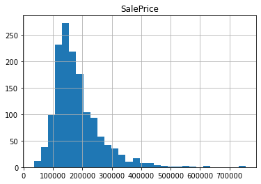
It wouldn’t be a bad idea to apply Box-Cox if using a linear model.
# we should make sure that no SalePrice values are missing
df.SalePrice.isna().any()
False
# it's also important to look at the degree of missingness in each of your features
column_missingness = df.isna().sum().sort_values(ascending=False) / len(df)
column_missingness.head(15)
PoolQC          0.995205
MiscFeature     0.963014
Alley           0.937671
Fence           0.807534
FireplaceQu     0.472603
LotFrontage     0.177397
GarageYrBlt     0.055479
GarageCond      0.055479
GarageType      0.055479
GarageFinish    0.055479
GarageQual      0.055479
BsmtFinType2    0.026027
BsmtExposure    0.026027
BsmtQual        0.025342
BsmtCond        0.025342
dtype: float64
Let’s go ahead and drop PoolQC, MiscFeature, and Alley as these are almost always missing. Note that some of these should be treated with more nuance. Take Fence for instance. I expect Fence takes the value NA when no fence is present.
features_to_drop = ['PoolQC', 'MiscFeature', 'Alley']
df = df.drop(features_to_drop, axis=1)
features = features[~features.variable.isin(features_to_drop)]
df.shape, features.shape
((1460, 78), (77, 3))
# Let's see if any rows are missing a large portion of their data
row_missingness = df.isna().sum(axis=1).sort_values(ascending=False) / len(df.columns)
row_missingness
39      0.153846
533     0.153846
520     0.153846
1011    0.153846
1218    0.153846
          ...
860     0.000000
51      0.000000
1170    0.000000
642     0.000000
810     0.000000
Length: 1460, dtype: float64
# let's take a closer look at some of these
index=39
df.loc[index, df.loc[index].isna()]
BsmtQual        NaN
BsmtCond        NaN
BsmtExposure    NaN
BsmtFinType1    NaN
BsmtFinType2    NaN
FireplaceQu     NaN
GarageType      NaN
GarageYrBlt     NaN
GarageFinish    NaN
GarageQual      NaN
GarageCond      NaN
Fence           NaN
Name: 39, dtype: object
Nothing too concerning here. Most of these features are very niche.
# get lists of categorical and numeric features
categorical_features = features.variable[features.type=='categorical'].tolist()
numeric_features = features.variable[features.type=='numeric'].tolist()[1:]
len(categorical_features), len(numeric_features)
(42, 34)
# let's take a look at our categorical features
categorical_features
['MSSubClass',
 'MSZoning',
 'Street',
 'LotShape',
 'LandContour',
 'Utilities',
 'LotConfig',
 'LandSlope',
 'Neighborhood',
 'Condition1',
 'Condition2',
 'BldgType',
 'HouseStyle',
 'RoofStyle',
 'RoofMatl',
 'Exterior1st',
 'Exterior2nd',
 'MasVnrType',
 'ExterQual',
 'ExterCond',
 'Foundation',
 'BsmtQual',
 'BsmtCond',
 'BsmtExposure',
 'BsmtFinType1',
 'BsmtFinType2',
 'Heating',
 'HeatingQC',
 'CentralAir',
 'Electrical',
 'KitchenQual',
 'Functional',
 'Fireplaces',
 'FireplaceQu',
 'GarageType',
 'GarageFinish',
 'GarageQual',
 'GarageCond',
 'PavedDrive',
 'Fence',
 'SaleType',
 'SaleCondition']
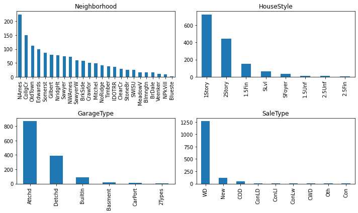
# Let's look at the distribution of features
plot_features = ['Neighborhood', 'HouseStyle', 'GarageType', 'SaleType']
fig, axes = plt.subplots(2,2)
fig.set_size_inches(10,6)
axes = axes.flatten()
for ix, feature in enumerate(plot_features):
    df[feature].value_counts().plot(kind='bar', ax=axes[ix])
    axes[ix].set_title(feature)
plt.tight_layout()
# let's take a look at our categorical features
numeric_features
['LotFrontage',
 'LotArea',
 'OverallQual',
 'OverallCond',
 'YearBuilt',
 'YearRemodAdd',
 'MasVnrArea',
 'BsmtFinSF1',
 'BsmtFinSF2',
 'BsmtUnfSF',
 'TotalBsmtSF',
 '1stFlrSF',
 '2ndFlrSF',
 'LowQualFinSF',
 'GrLivArea',
 'BsmtFullBath',
 'BsmtHalfBath',
 'FullBath',
 'HalfBath',
 'BedroomAbvGr',
 'KitchenAbvGr',
 'TotRmsAbvGrd',
 'GarageYrBlt',
 'GarageCars',
 'GarageArea',
 'WoodDeckSF',
 'OpenPorchSF',
 'EnclosedPorch',
 '3SsnPorch',
 'ScreenPorch',
 'PoolArea',
 'MiscVal',
 'MoSold',
 'YrSold']
# since these are numeric, we can compute some basic stats:
df[numeric_features].describe()
| LotFrontage | LotArea | OverallQual | OverallCond | YearBuilt | YearRemodAdd | MasVnrArea | BsmtFinSF1 | BsmtFinSF2 | BsmtUnfSF | ... | GarageArea | WoodDeckSF | OpenPorchSF | EnclosedPorch | 3SsnPorch | ScreenPorch | PoolArea | MiscVal | MoSold | YrSold | |
|---|---|---|---|---|---|---|---|---|---|---|---|---|---|---|---|---|---|---|---|---|---|
| count | 1201.000000 | 1460.000000 | 1460.000000 | 1460.000000 | 1460.000000 | 1460.000000 | 1452.000000 | 1460.000000 | 1460.000000 | 1460.000000 | ... | 1460.000000 | 1460.000000 | 1460.000000 | 1460.000000 | 1460.000000 | 1460.000000 | 1460.000000 | 1460.000000 | 1460.000000 | 1460.000000 |
| mean | 70.049958 | 10516.828082 | 6.099315 | 5.575342 | 1971.267808 | 1984.865753 | 103.685262 | 443.639726 | 46.549315 | 567.240411 | ... | 472.980137 | 94.244521 | 46.660274 | 21.954110 | 3.409589 | 15.060959 | 2.758904 | 43.489041 | 6.321918 | 2007.815753 |
| std | 24.284752 | 9981.264932 | 1.382997 | 1.112799 | 30.202904 | 20.645407 | 181.066207 | 456.098091 | 161.319273 | 441.866955 | ... | 213.804841 | 125.338794 | 66.256028 | 61.119149 | 29.317331 | 55.757415 | 40.177307 | 496.123024 | 2.703626 | 1.328095 |
| min | 21.000000 | 1300.000000 | 1.000000 | 1.000000 | 1872.000000 | 1950.000000 | 0.000000 | 0.000000 | 0.000000 | 0.000000 | ... | 0.000000 | 0.000000 | 0.000000 | 0.000000 | 0.000000 | 0.000000 | 0.000000 | 0.000000 | 1.000000 | 2006.000000 |
| 25% | 59.000000 | 7553.500000 | 5.000000 | 5.000000 | 1954.000000 | 1967.000000 | 0.000000 | 0.000000 | 0.000000 | 223.000000 | ... | 334.500000 | 0.000000 | 0.000000 | 0.000000 | 0.000000 | 0.000000 | 0.000000 | 0.000000 | 5.000000 | 2007.000000 |
| 50% | 69.000000 | 9478.500000 | 6.000000 | 5.000000 | 1973.000000 | 1994.000000 | 0.000000 | 383.500000 | 0.000000 | 477.500000 | ... | 480.000000 | 0.000000 | 25.000000 | 0.000000 | 0.000000 | 0.000000 | 0.000000 | 0.000000 | 6.000000 | 2008.000000 |
| 75% | 80.000000 | 11601.500000 | 7.000000 | 6.000000 | 2000.000000 | 2004.000000 | 166.000000 | 712.250000 | 0.000000 | 808.000000 | ... | 576.000000 | 168.000000 | 68.000000 | 0.000000 | 0.000000 | 0.000000 | 0.000000 | 0.000000 | 8.000000 | 2009.000000 |
| max | 313.000000 | 215245.000000 | 10.000000 | 9.000000 | 2010.000000 | 2010.000000 | 1600.000000 | 5644.000000 | 1474.000000 | 2336.000000 | ... | 1418.000000 | 857.000000 | 547.000000 | 552.000000 | 508.000000 | 480.000000 | 738.000000 | 15500.000000 | 12.000000 | 2010.000000 |
8 rows × 34 columns
Probably, most of these should be rescaled with standard scaling.
# Let's look at the distribution of features
plot_features = ['LotFrontage', 'BsmtFinSF1', '1stFlrSF', 'ScreenPorch']
fig, axes = plt.subplots(2,2)
fig.set_size_inches(10,6)
axes = axes.flatten()
for ix, feature in enumerate(plot_features):
    df[feature].value_counts().plot(kind='hist', ax=axes[ix], bins=20, logy=True)
    axes[ix].set_title(feature)
plt.tight_layout()
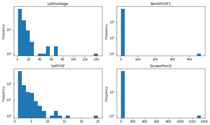
Some of these features have very low variance. They should probably be removed. Others should possibly be transformed using Box-Cox or similar.
# Let's check to see if any of our numeric features are highly correlated with one another
import seaborn as sns
plt.gcf().set_size_inches(10,8)
sns.clustermap(df[numeric_features].corr())
<seaborn.matrix.ClusterGrid at 0x15448283b5e0>
<Figure size 720x576 with 0 Axes>
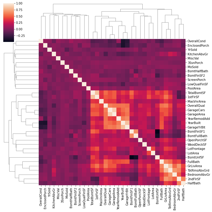
Overall, our features are relatively uncorrelated. Some features are highly correlated. For instance:
TotalBsmtSF, 1stFlrSF
GarageCars, GarageArea
BsmtFnSF1, BsmtFullBath
We could consider removing some of these near duplicate features.
First pass#
It’s usually a good idea to first perform a quick and dirty analysis ignoring the subtleties that we discussed above. We can then try to incorporate these ideas to improve our results.
# define input/target
inputs = features.variable.iloc[1:].tolist()
X, y = df[inputs], df['SalePrice']
X.shape, y.shape
((1460, 76), (1460,))
# split the data
from sklearn.model_selection import train_test_split
X_train, X_test, y_train, y_test = train_test_split(X, y, test_size=0.2, shuffle=True, random_state=42)
X_train.shape, X_test.shape
((1168, 76), (292, 76))
Preprocessing numeric and categorical features#
We will use scikit-learn’s pipeline feature to streamline the model fitting and evaluation process.
from sklearn.preprocessing import StandardScaler, OneHotEncoder
from sklearn.impute import SimpleImputer
from sklearn.pipeline import Pipeline
from sklearn.compose import make_column_transformer, ColumnTransformer

# preprocessing pipeline for numeric quantities
preproc_numeric = Pipeline([
    ('fill_na', SimpleImputer(strategy='median')),
    ('scale', StandardScaler())
])

# preprocessing pipeline for categorical quantities
preproc_categorical = Pipeline([
    ('fill_na', SimpleImputer(strategy='most_frequent')),
    ('encode', OneHotEncoder(sparse_output=False, drop='first', min_frequency=5, handle_unknown='infrequent_if_exist'))
])

# full preprocessing pipeline
preproc = ColumnTransformer(
    transformers=[
    ('numeric', preproc_numeric, numeric_features),
    ('categorical', preproc_categorical, categorical_features)
], verbose_feature_names_out=False)

preproc.fit(X_train)
ColumnTransformer(transformers=[('numeric',
                                 Pipeline(steps=[('fill_na',
                                                  SimpleImputer(strategy='median')),
                                                 ('scale', StandardScaler())]),
                                 ['LotFrontage', 'LotArea', 'OverallQual',
                                  'OverallCond', 'YearBuilt', 'YearRemodAdd',
                                  'MasVnrArea', 'BsmtFinSF1', 'BsmtFinSF2',
                                  'BsmtUnfSF', 'TotalBsmtSF', '1stFlrSF',
                                  '2ndFlrSF', 'LowQualFinSF', 'GrLivArea',
                                  'BsmtFullBath', 'BsmtHal...
                                  'LotShape', 'LandContour', 'Utilities',
                                  'LotConfig', 'LandSlope', 'Neighborhood',
                                  'Condition1', 'Condition2', 'BldgType',
                                  'HouseStyle', 'RoofStyle', 'RoofMatl',
                                  'Exterior1st', 'Exterior2nd', 'MasVnrType',
                                  'ExterQual', 'ExterCond', 'Foundation',
                                  'BsmtQual', 'BsmtCond', 'BsmtExposure',
                                  'BsmtFinType1', 'BsmtFinType2', 'Heating',
                                  'HeatingQC', 'CentralAir', 'Electrical', ...])],
                  verbose_feature_names_out=False)
In a Jupyter environment, please rerun this cell to show the HTML representation or trust the notebook. On GitHub, the HTML representation is unable to render, please try loading this page with nbviewer.org.
ColumnTransformer(transformers=[('numeric',
                                 Pipeline(steps=[('fill_na',
                                                  SimpleImputer(strategy='median')),
                                                 ('scale', StandardScaler())]),
                                 ['LotFrontage', 'LotArea', 'OverallQual',
                                  'OverallCond', 'YearBuilt', 'YearRemodAdd',
                                  'MasVnrArea', 'BsmtFinSF1', 'BsmtFinSF2',
                                  'BsmtUnfSF', 'TotalBsmtSF', '1stFlrSF',
                                  '2ndFlrSF', 'LowQualFinSF', 'GrLivArea',
                                  'BsmtFullBath', 'BsmtHal...
                                  'LotShape', 'LandContour', 'Utilities',
                                  'LotConfig', 'LandSlope', 'Neighborhood',
                                  'Condition1', 'Condition2', 'BldgType',
                                  'HouseStyle', 'RoofStyle', 'RoofMatl',
                                  'Exterior1st', 'Exterior2nd', 'MasVnrType',
                                  'ExterQual', 'ExterCond', 'Foundation',
                                  'BsmtQual', 'BsmtCond', 'BsmtExposure',
                                  'BsmtFinType1', 'BsmtFinType2', 'Heating',
                                  'HeatingQC', 'CentralAir', 'Electrical', ...])],
verbose_feature_names_out=False)['LotFrontage', 'LotArea', 'OverallQual', 'OverallCond', 'YearBuilt', 'YearRemodAdd', 'MasVnrArea', 'BsmtFinSF1', 'BsmtFinSF2', 'BsmtUnfSF', 'TotalBsmtSF', '1stFlrSF', '2ndFlrSF', 'LowQualFinSF', 'GrLivArea', 'BsmtFullBath', 'BsmtHalfBath', 'FullBath', 'HalfBath', 'BedroomAbvGr', 'KitchenAbvGr', 'TotRmsAbvGrd', 'GarageYrBlt', 'GarageCars', 'GarageArea', 'WoodDeckSF', 'OpenPorchSF', 'EnclosedPorch', '3SsnPorch', 'ScreenPorch', 'PoolArea', 'MiscVal', 'MoSold', 'YrSold']
SimpleImputer(strategy='median')
StandardScaler()
['MSSubClass', 'MSZoning', 'Street', 'LotShape', 'LandContour', 'Utilities', 'LotConfig', 'LandSlope', 'Neighborhood', 'Condition1', 'Condition2', 'BldgType', 'HouseStyle', 'RoofStyle', 'RoofMatl', 'Exterior1st', 'Exterior2nd', 'MasVnrType', 'ExterQual', 'ExterCond', 'Foundation', 'BsmtQual', 'BsmtCond', 'BsmtExposure', 'BsmtFinType1', 'BsmtFinType2', 'Heating', 'HeatingQC', 'CentralAir', 'Electrical', 'KitchenQual', 'Functional', 'Fireplaces', 'FireplaceQu', 'GarageType', 'GarageFinish', 'GarageQual', 'GarageCond', 'PavedDrive', 'Fence', 'SaleType', 'SaleCondition']
SimpleImputer(strategy='most_frequent')
OneHotEncoder(drop='first', handle_unknown='infrequent_if_exist',
min_frequency=5, sparse_output=False)preproc.transform(X_test)
| LotFrontage | LotArea | OverallQual | OverallCond | YearBuilt | YearRemodAdd | MasVnrArea | BsmtFinSF1 | BsmtFinSF2 | BsmtUnfSF | ... | Fence_MnWw | SaleType_ConLD | SaleType_New | SaleType_WD | SaleType_infrequent_sklearn | SaleCondition_Alloca | SaleCondition_Family | SaleCondition_Normal | SaleCondition_Partial | SaleCondition_infrequent_sklearn | |
|---|---|---|---|---|---|---|---|---|---|---|---|---|---|---|---|---|---|---|---|---|---|
| 892 | -0.012468 | -0.211594 | -0.088934 | 2.165000 | -0.259789 | 0.873470 | -0.597889 | 0.472844 | -0.285504 | -0.391317 | ... | 0.0 | 0.0 | 0.0 | 1.0 | 0.0 | 0.0 | 0.0 | 1.0 | 0.0 | 0.0 |
| 1105 | 1.234520 | 0.145643 | 1.374088 | -0.524174 | 0.751222 | 0.487465 | 1.498567 | 1.276986 | -0.285504 | -0.312872 | ... | 0.0 | 0.0 | 0.0 | 1.0 | 0.0 | 0.0 | 0.0 | 1.0 | 0.0 | 0.0 |
| 413 | -0.635963 | -0.160826 | -0.820445 | 0.372217 | -1.433867 | -1.683818 | -0.597889 | -0.971996 | -0.285504 | 0.980347 | ... | 0.0 | 0.0 | 0.0 | 1.0 | 0.0 | 0.0 | 0.0 | 1.0 | 0.0 | 0.0 |
| 522 | -0.903175 | -0.529035 | -0.088934 | 1.268609 | -0.781602 | -1.683818 | -0.597889 | -0.102477 | -0.285504 | 0.077111 | ... | 0.0 | 0.0 | 0.0 | 1.0 | 0.0 | 0.0 | 0.0 | 1.0 | 0.0 | 0.0 |
| 1036 | 0.833703 | 0.205338 | 2.105599 | -0.524174 | 1.175195 | 1.114724 | -0.192497 | 1.255193 | -0.285504 | 0.061422 | ... | 0.0 | 0.0 | 0.0 | 1.0 | 0.0 | 0.0 | 0.0 | 1.0 | 0.0 | 0.0 |
| ... | ... | ... | ... | ... | ... | ... | ... | ... | ... | ... | ... | ... | ... | ... | ... | ... | ... | ... | ... | ... | ... |
| 479 | -0.903175 | -0.443026 | -1.551955 | 1.268609 | -1.107734 | 0.728718 | 1.921333 | -0.605882 | -0.285504 | 0.377443 | ... | 0.0 | 0.0 | 0.0 | 1.0 | 0.0 | 1.0 | 0.0 | 0.0 | 0.0 | 0.0 |
| 1361 | 2.392439 | 0.508459 | 0.642577 | -0.524174 | 1.109968 | 0.969972 | -0.505228 | 1.804363 | -0.285504 | -0.705096 | ... | 0.0 | 0.0 | 0.0 | 1.0 | 0.0 | 0.0 | 0.0 | 1.0 | 0.0 | 0.0 |
| 802 | -0.324216 | -0.231585 | 0.642577 | -0.524174 | 1.109968 | 0.969972 | -0.597889 | 0.440155 | -0.285504 | -1.099561 | ... | 0.0 | 0.0 | 0.0 | 1.0 | 0.0 | 0.0 | 0.0 | 1.0 | 0.0 | 0.0 |
| 651 | -0.457822 | -0.149296 | -1.551955 | -0.524174 | -1.009895 | -1.683818 | -0.597889 | -0.971996 | -0.285504 | 0.413303 | ... | 0.0 | 0.0 | 0.0 | 1.0 | 0.0 | 0.0 | 0.0 | 1.0 | 0.0 | 0.0 |
| 722 | -0.012468 | -0.238931 | -1.551955 | 1.268609 | -0.031496 | -0.718804 | -0.597889 | -0.555760 | -0.285504 | 0.229518 | ... | 0.0 | 0.0 | 0.0 | 1.0 | 0.0 | 0.0 | 0.0 | 1.0 | 0.0 | 0.0 |
292 rows × 226 columns
Model fitting#
# create the model pipeline
from sklearn.linear_model import Ridge

pipe = Pipeline([
    ('preproc', preproc),
    ('estimator', Ridge(alpha=1))
])

# fit
pipe.fit(X_train, y_train)
Pipeline(steps=[('preproc',
                 ColumnTransformer(transformers=[('numeric',
                                                  Pipeline(steps=[('fill_na',
                                                                   SimpleImputer(strategy='median')),
                                                                  ('scale',
                                                                   StandardScaler())]),
                                                  ['LotFrontage', 'LotArea',
                                                   'OverallQual', 'OverallCond',
                                                   'YearBuilt', 'YearRemodAdd',
                                                   'MasVnrArea', 'BsmtFinSF1',
                                                   'BsmtFinSF2', 'BsmtUnfSF',
                                                   'TotalBsmtSF', '1stFlrSF',
                                                   '2ndFlrSF', 'LowQualFinSF',
                                                   'GrLivAr...
                                                   'Neighborhood', 'Condition1',
                                                   'Condition2', 'BldgType',
                                                   'HouseStyle', 'RoofStyle',
                                                   'RoofMatl', 'Exterior1st',
                                                   'Exterior2nd', 'MasVnrType',
                                                   'ExterQual', 'ExterCond',
                                                   'Foundation', 'BsmtQual',
                                                   'BsmtCond', 'BsmtExposure',
                                                   'BsmtFinType1',
                                                   'BsmtFinType2', 'Heating',
                                                   'HeatingQC', 'CentralAir',
                                                   'Electrical', ...])],
                                   verbose_feature_names_out=False)),
                ('estimator', Ridge(alpha=1))])
In a Jupyter environment, please rerun this cell to show the HTML representation or trust the notebook. On GitHub, the HTML representation is unable to render, please try loading this page with nbviewer.org.
Pipeline(steps=[('preproc',
                 ColumnTransformer(transformers=[('numeric',
                                                  Pipeline(steps=[('fill_na',
                                                                   SimpleImputer(strategy='median')),
                                                                  ('scale',
                                                                   StandardScaler())]),
                                                  ['LotFrontage', 'LotArea',
                                                   'OverallQual', 'OverallCond',
                                                   'YearBuilt', 'YearRemodAdd',
                                                   'MasVnrArea', 'BsmtFinSF1',
                                                   'BsmtFinSF2', 'BsmtUnfSF',
                                                   'TotalBsmtSF', '1stFlrSF',
                                                   '2ndFlrSF', 'LowQualFinSF',
                                                   'GrLivAr...
                                                   'Neighborhood', 'Condition1',
                                                   'Condition2', 'BldgType',
                                                   'HouseStyle', 'RoofStyle',
                                                   'RoofMatl', 'Exterior1st',
                                                   'Exterior2nd', 'MasVnrType',
                                                   'ExterQual', 'ExterCond',
                                                   'Foundation', 'BsmtQual',
                                                   'BsmtCond', 'BsmtExposure',
                                                   'BsmtFinType1',
                                                   'BsmtFinType2', 'Heating',
                                                   'HeatingQC', 'CentralAir',
                                                   'Electrical', ...])],
                                   verbose_feature_names_out=False)),
('estimator', Ridge(alpha=1))])ColumnTransformer(transformers=[('numeric',
Pipeline(steps=[('fill_na',
SimpleImputer(strategy='median')),
('scale', StandardScaler())]),
['LotFrontage', 'LotArea', 'OverallQual',
'OverallCond', 'YearBuilt', 'YearRemodAdd',
'MasVnrArea', 'BsmtFinSF1', 'BsmtFinSF2',
'BsmtUnfSF', 'TotalBsmtSF', '1stFlrSF',
'2ndFlrSF', 'LowQualFinSF', 'GrLivArea',
'BsmtFullBath', 'BsmtHal...
'LotShape', 'LandContour', 'Utilities',
'LotConfig', 'LandSlope', 'Neighborhood',
'Condition1', 'Condition2', 'BldgType',
'HouseStyle', 'RoofStyle', 'RoofMatl',
'Exterior1st', 'Exterior2nd', 'MasVnrType',
'ExterQual', 'ExterCond', 'Foundation',
'BsmtQual', 'BsmtCond', 'BsmtExposure',
'BsmtFinType1', 'BsmtFinType2', 'Heating',
'HeatingQC', 'CentralAir', 'Electrical', ...])],
verbose_feature_names_out=False)['LotFrontage', 'LotArea', 'OverallQual', 'OverallCond', 'YearBuilt', 'YearRemodAdd', 'MasVnrArea', 'BsmtFinSF1', 'BsmtFinSF2', 'BsmtUnfSF', 'TotalBsmtSF', '1stFlrSF', '2ndFlrSF', 'LowQualFinSF', 'GrLivArea', 'BsmtFullBath', 'BsmtHalfBath', 'FullBath', 'HalfBath', 'BedroomAbvGr', 'KitchenAbvGr', 'TotRmsAbvGrd', 'GarageYrBlt', 'GarageCars', 'GarageArea', 'WoodDeckSF', 'OpenPorchSF', 'EnclosedPorch', '3SsnPorch', 'ScreenPorch', 'PoolArea', 'MiscVal', 'MoSold', 'YrSold']
SimpleImputer(strategy='median')
StandardScaler()
['MSSubClass', 'MSZoning', 'Street', 'LotShape', 'LandContour', 'Utilities', 'LotConfig', 'LandSlope', 'Neighborhood', 'Condition1', 'Condition2', 'BldgType', 'HouseStyle', 'RoofStyle', 'RoofMatl', 'Exterior1st', 'Exterior2nd', 'MasVnrType', 'ExterQual', 'ExterCond', 'Foundation', 'BsmtQual', 'BsmtCond', 'BsmtExposure', 'BsmtFinType1', 'BsmtFinType2', 'Heating', 'HeatingQC', 'CentralAir', 'Electrical', 'KitchenQual', 'Functional', 'Fireplaces', 'FireplaceQu', 'GarageType', 'GarageFinish', 'GarageQual', 'GarageCond', 'PavedDrive', 'Fence', 'SaleType', 'SaleCondition']
SimpleImputer(strategy='most_frequent')
OneHotEncoder(drop='first', handle_unknown='infrequent_if_exist',
min_frequency=5, sparse_output=False)Ridge(alpha=1)
Model evaluation#
# evaluate
# For random forest regressor, score returns the R^2 value
print("Train R^2:", pipe.score(X_train, y_train))
print("Test R^2:", pipe.score(X_test, y_test))
Train R^2: 0.9028881797596011
Test R^2: 0.8714648323729995
# MAE is a more intuitive metric for price estimation
from sklearn.metrics import mean_absolute_error
y_train_pred_1stpass = pipe.predict(X_train)
y_test_pred_1stpass = pipe.predict(X_test)
print("Train MAE:", mean_absolute_error(y_train, y_train_pred_1stpass))
print("Test MAE:", mean_absolute_error(y_test, y_test_pred_1stpass))
Train MAE: 15288.339516024189
Test MAE: 20544.401602914677
# more robust classification with cross validation
from sklearn.model_selection import KFold, cross_validate
cv = KFold(n_splits=5, shuffle=True, random_state=42)
cv_scores = cross_validate(pipe, X, y, n_jobs=4, return_train_score=True, scoring='neg_mean_absolute_error')
cv_scores
{'fit_time': array([0.16545057, 0.14652419, 0.1494379 , 0.14467359, 0.12987018]),
 'score_time': array([0.03685045, 0.03611279, 0.03650355, 0.03635812, 0.03367758]),
 'test_score': array([-18480.22849655, -20702.55584883, -20390.70685371, -17442.23199009,
        -19762.00113844]),
 'train_score': array([-15920.87447649, -14995.07168281, -15245.2950543 , -15810.8980323 ,
        -13704.36598872])}
import scipy
def mean_confidence_interval(data, confidence=0.95):
    a = 1.0 * np.array(data)
    n = len(a)
    m, se = np.mean(a), scipy.stats.sem(a)
    h = se * scipy.stats.t.ppf((1 + confidence) / 2., n-1)
    return m, (m-h, m+h)

mean_confidence_interval(-cv_scores['test_score'])
(19355.544865524786, (17657.804810833954, 21053.284920215618))
Optimizing the pipeline#
There are many things we can try to improve the fit of our model. For example, we could experiment with the following:
apply some of the observations from our exploratory data analysis
different imputation strategies
add a dimension reduction step like PCA
try different estimators
try hyperparameters within different estimators
How do we start testing various approaches in scikit-learn? One way is to manually change the pipeline we defined above, fit/evaluate the model, and compare with our results above. This can be a tedious and error-prone process. Let’s see how do this efficiently using scikit-learn’s APIs.
To introduce the ideas, let’s consider the alpha regularization parameter used in Ridge regression.
Tuning estimator parameters#
pipe
Pipeline(steps=[('preproc',
                 ColumnTransformer(transformers=[('numeric',
                                                  Pipeline(steps=[('fill_na',
                                                                   SimpleImputer(strategy='median')),
                                                                  ('scale',
                                                                   StandardScaler())]),
                                                  ['LotFrontage', 'LotArea',
                                                   'OverallQual', 'OverallCond',
                                                   'YearBuilt', 'YearRemodAdd',
                                                   'MasVnrArea', 'BsmtFinSF1',
                                                   'BsmtFinSF2', 'BsmtUnfSF',
                                                   'TotalBsmtSF', '1stFlrSF',
                                                   '2ndFlrSF', 'LowQualFinSF',
                                                   'GrLivAr...
                                                   'Neighborhood', 'Condition1',
                                                   'Condition2', 'BldgType',
                                                   'HouseStyle', 'RoofStyle',
                                                   'RoofMatl', 'Exterior1st',
                                                   'Exterior2nd', 'MasVnrType',
                                                   'ExterQual', 'ExterCond',
                                                   'Foundation', 'BsmtQual',
                                                   'BsmtCond', 'BsmtExposure',
                                                   'BsmtFinType1',
                                                   'BsmtFinType2', 'Heating',
                                                   'HeatingQC', 'CentralAir',
                                                   'Electrical', ...])],
                                   verbose_feature_names_out=False)),
                ('estimator', Ridge(alpha=1))])
In a Jupyter environment, please rerun this cell to show the HTML representation or trust the notebook. On GitHub, the HTML representation is unable to render, please try loading this page with nbviewer.org.
Pipeline(steps=[('preproc',
                 ColumnTransformer(transformers=[('numeric',
                                                  Pipeline(steps=[('fill_na',
                                                                   SimpleImputer(strategy='median')),
                                                                  ('scale',
                                                                   StandardScaler())]),
                                                  ['LotFrontage', 'LotArea',
                                                   'OverallQual', 'OverallCond',
                                                   'YearBuilt', 'YearRemodAdd',
                                                   'MasVnrArea', 'BsmtFinSF1',
                                                   'BsmtFinSF2', 'BsmtUnfSF',
                                                   'TotalBsmtSF', '1stFlrSF',
                                                   '2ndFlrSF', 'LowQualFinSF',
                                                   'GrLivAr...
                                                   'Neighborhood', 'Condition1',
                                                   'Condition2', 'BldgType',
                                                   'HouseStyle', 'RoofStyle',
                                                   'RoofMatl', 'Exterior1st',
                                                   'Exterior2nd', 'MasVnrType',
                                                   'ExterQual', 'ExterCond',
                                                   'Foundation', 'BsmtQual',
                                                   'BsmtCond', 'BsmtExposure',
                                                   'BsmtFinType1',
                                                   'BsmtFinType2', 'Heating',
                                                   'HeatingQC', 'CentralAir',
                                                   'Electrical', ...])],
                                   verbose_feature_names_out=False)),
('estimator', Ridge(alpha=1))])ColumnTransformer(transformers=[('numeric',
Pipeline(steps=[('fill_na',
SimpleImputer(strategy='median')),
('scale', StandardScaler())]),
['LotFrontage', 'LotArea', 'OverallQual',
'OverallCond', 'YearBuilt', 'YearRemodAdd',
'MasVnrArea', 'BsmtFinSF1', 'BsmtFinSF2',
'BsmtUnfSF', 'TotalBsmtSF', '1stFlrSF',
'2ndFlrSF', 'LowQualFinSF', 'GrLivArea',
'BsmtFullBath', 'BsmtHal...
'LotShape', 'LandContour', 'Utilities',
'LotConfig', 'LandSlope', 'Neighborhood',
'Condition1', 'Condition2', 'BldgType',
'HouseStyle', 'RoofStyle', 'RoofMatl',
'Exterior1st', 'Exterior2nd', 'MasVnrType',
'ExterQual', 'ExterCond', 'Foundation',
'BsmtQual', 'BsmtCond', 'BsmtExposure',
'BsmtFinType1', 'BsmtFinType2', 'Heating',
'HeatingQC', 'CentralAir', 'Electrical', ...])],
verbose_feature_names_out=False)['LotFrontage', 'LotArea', 'OverallQual', 'OverallCond', 'YearBuilt', 'YearRemodAdd', 'MasVnrArea', 'BsmtFinSF1', 'BsmtFinSF2', 'BsmtUnfSF', 'TotalBsmtSF', '1stFlrSF', '2ndFlrSF', 'LowQualFinSF', 'GrLivArea', 'BsmtFullBath', 'BsmtHalfBath', 'FullBath', 'HalfBath', 'BedroomAbvGr', 'KitchenAbvGr', 'TotRmsAbvGrd', 'GarageYrBlt', 'GarageCars', 'GarageArea', 'WoodDeckSF', 'OpenPorchSF', 'EnclosedPorch', '3SsnPorch', 'ScreenPorch', 'PoolArea', 'MiscVal', 'MoSold', 'YrSold']
SimpleImputer(strategy='median')
StandardScaler()
['MSSubClass', 'MSZoning', 'Street', 'LotShape', 'LandContour', 'Utilities', 'LotConfig', 'LandSlope', 'Neighborhood', 'Condition1', 'Condition2', 'BldgType', 'HouseStyle', 'RoofStyle', 'RoofMatl', 'Exterior1st', 'Exterior2nd', 'MasVnrType', 'ExterQual', 'ExterCond', 'Foundation', 'BsmtQual', 'BsmtCond', 'BsmtExposure', 'BsmtFinType1', 'BsmtFinType2', 'Heating', 'HeatingQC', 'CentralAir', 'Electrical', 'KitchenQual', 'Functional', 'Fireplaces', 'FireplaceQu', 'GarageType', 'GarageFinish', 'GarageQual', 'GarageCond', 'PavedDrive', 'Fence', 'SaleType', 'SaleCondition']
SimpleImputer(strategy='most_frequent')
OneHotEncoder(drop='first', handle_unknown='infrequent_if_exist',
min_frequency=5, sparse_output=False)Ridge(alpha=1)
from sklearn.model_selection import GridSearchCV
alphas = np.logspace(-2,3,10)
param_grid = {
    'estimator__alpha': alphas
}
cv = KFold(10, shuffle=True)
gs = GridSearchCV(pipe, param_grid, cv=cv, n_jobs=10, scoring='neg_mean_absolute_error', verbose=False)

gs.fit(X_train, y_train)
gs.best_estimator_
Pipeline(steps=[('preproc',
                 ColumnTransformer(transformers=[('numeric',
                                                  Pipeline(steps=[('fill_na',
                                                                   SimpleImputer(strategy='median')),
                                                                  ('scale',
                                                                   StandardScaler())]),
                                                  ['LotFrontage', 'LotArea',
                                                   'OverallQual', 'OverallCond',
                                                   'YearBuilt', 'YearRemodAdd',
                                                   'MasVnrArea', 'BsmtFinSF1',
                                                   'BsmtFinSF2', 'BsmtUnfSF',
                                                   'TotalBsmtSF', '1stFlrSF',
                                                   '2ndFlrSF', 'LowQualFinSF',
                                                   'GrLivAr...
                                                   'Neighborhood', 'Condition1',
                                                   'Condition2', 'BldgType',
                                                   'HouseStyle', 'RoofStyle',
                                                   'RoofMatl', 'Exterior1st',
                                                   'Exterior2nd', 'MasVnrType',
                                                   'ExterQual', 'ExterCond',
                                                   'Foundation', 'BsmtQual',
                                                   'BsmtCond', 'BsmtExposure',
                                                   'BsmtFinType1',
                                                   'BsmtFinType2', 'Heating',
                                                   'HeatingQC', 'CentralAir',
                                                   'Electrical', ...])],
                                   verbose_feature_names_out=False)),
                ('estimator', Ridge(alpha=21.544346900318846))])
In a Jupyter environment, please rerun this cell to show the HTML representation or trust the notebook. On GitHub, the HTML representation is unable to render, please try loading this page with nbviewer.org.
Pipeline(steps=[('preproc',
                 ColumnTransformer(transformers=[('numeric',
                                                  Pipeline(steps=[('fill_na',
                                                                   SimpleImputer(strategy='median')),
                                                                  ('scale',
                                                                   StandardScaler())]),
                                                  ['LotFrontage', 'LotArea',
                                                   'OverallQual', 'OverallCond',
                                                   'YearBuilt', 'YearRemodAdd',
                                                   'MasVnrArea', 'BsmtFinSF1',
                                                   'BsmtFinSF2', 'BsmtUnfSF',
                                                   'TotalBsmtSF', '1stFlrSF',
                                                   '2ndFlrSF', 'LowQualFinSF',
                                                   'GrLivAr...
                                                   'Neighborhood', 'Condition1',
                                                   'Condition2', 'BldgType',
                                                   'HouseStyle', 'RoofStyle',
                                                   'RoofMatl', 'Exterior1st',
                                                   'Exterior2nd', 'MasVnrType',
                                                   'ExterQual', 'ExterCond',
                                                   'Foundation', 'BsmtQual',
                                                   'BsmtCond', 'BsmtExposure',
                                                   'BsmtFinType1',
                                                   'BsmtFinType2', 'Heating',
                                                   'HeatingQC', 'CentralAir',
                                                   'Electrical', ...])],
                                   verbose_feature_names_out=False)),
('estimator', Ridge(alpha=21.544346900318846))])ColumnTransformer(transformers=[('numeric',
Pipeline(steps=[('fill_na',
SimpleImputer(strategy='median')),
('scale', StandardScaler())]),
['LotFrontage', 'LotArea', 'OverallQual',
'OverallCond', 'YearBuilt', 'YearRemodAdd',
'MasVnrArea', 'BsmtFinSF1', 'BsmtFinSF2',
'BsmtUnfSF', 'TotalBsmtSF', '1stFlrSF',
'2ndFlrSF', 'LowQualFinSF', 'GrLivArea',
'BsmtFullBath', 'BsmtHal...
'LotShape', 'LandContour', 'Utilities',
'LotConfig', 'LandSlope', 'Neighborhood',
'Condition1', 'Condition2', 'BldgType',
'HouseStyle', 'RoofStyle', 'RoofMatl',
'Exterior1st', 'Exterior2nd', 'MasVnrType',
'ExterQual', 'ExterCond', 'Foundation',
'BsmtQual', 'BsmtCond', 'BsmtExposure',
'BsmtFinType1', 'BsmtFinType2', 'Heating',
'HeatingQC', 'CentralAir', 'Electrical', ...])],
verbose_feature_names_out=False)['LotFrontage', 'LotArea', 'OverallQual', 'OverallCond', 'YearBuilt', 'YearRemodAdd', 'MasVnrArea', 'BsmtFinSF1', 'BsmtFinSF2', 'BsmtUnfSF', 'TotalBsmtSF', '1stFlrSF', '2ndFlrSF', 'LowQualFinSF', 'GrLivArea', 'BsmtFullBath', 'BsmtHalfBath', 'FullBath', 'HalfBath', 'BedroomAbvGr', 'KitchenAbvGr', 'TotRmsAbvGrd', 'GarageYrBlt', 'GarageCars', 'GarageArea', 'WoodDeckSF', 'OpenPorchSF', 'EnclosedPorch', '3SsnPorch', 'ScreenPorch', 'PoolArea', 'MiscVal', 'MoSold', 'YrSold']
SimpleImputer(strategy='median')
StandardScaler()
['MSSubClass', 'MSZoning', 'Street', 'LotShape', 'LandContour', 'Utilities', 'LotConfig', 'LandSlope', 'Neighborhood', 'Condition1', 'Condition2', 'BldgType', 'HouseStyle', 'RoofStyle', 'RoofMatl', 'Exterior1st', 'Exterior2nd', 'MasVnrType', 'ExterQual', 'ExterCond', 'Foundation', 'BsmtQual', 'BsmtCond', 'BsmtExposure', 'BsmtFinType1', 'BsmtFinType2', 'Heating', 'HeatingQC', 'CentralAir', 'Electrical', 'KitchenQual', 'Functional', 'Fireplaces', 'FireplaceQu', 'GarageType', 'GarageFinish', 'GarageQual', 'GarageCond', 'PavedDrive', 'Fence', 'SaleType', 'SaleCondition']
SimpleImputer(strategy='most_frequent')
OneHotEncoder(drop='first', handle_unknown='infrequent_if_exist',
min_frequency=5, sparse_output=False)Ridge(alpha=21.544346900318846)
# look at the grid search outcome
gs.cv_results_
{'mean_fit_time': array([0.21524832, 0.12929206, 0.14147673, 0.13001094, 0.12876217,
        0.12753346, 0.12873785, 0.12855723, 0.12965353, 0.1284827 ]),
 'std_fit_time': array([0.03227405, 0.00410048, 0.0115528 , 0.00307046, 0.00154043,
        0.00228009, 0.00147471, 0.00239597, 0.00322923, 0.00289472]),
 'mean_score_time': array([0.03430345, 0.03392034, 0.03475215, 0.03282845, 0.03321393,
        0.03305686, 0.03315287, 0.03283639, 0.03680825, 0.03171299]),
 'std_score_time': array([0.00137619, 0.00102129, 0.00133493, 0.00081006, 0.00101256,
        0.00059905, 0.00092702, 0.00072003, 0.00701796, 0.00133118]),
 'param_estimator__alpha': masked_array(data=[0.01, 0.03593813663804628, 0.1291549665014884,
                    0.464158883361278, 1.6681005372000592,
                    5.994842503189409, 21.544346900318846,
                    77.42636826811278, 278.2559402207126, 1000.0],
              mask=[False, False, False, False, False, False, False, False,
                    False, False],
        fill_value='?',
             dtype=object),
 'params': [{'estimator__alpha': 0.01},
  {'estimator__alpha': 0.03593813663804628},
  {'estimator__alpha': 0.1291549665014884},
  {'estimator__alpha': 0.464158883361278},
  {'estimator__alpha': 1.6681005372000592},
  {'estimator__alpha': 5.994842503189409},
  {'estimator__alpha': 21.544346900318846},
  {'estimator__alpha': 77.42636826811278},
  {'estimator__alpha': 278.2559402207126},
  {'estimator__alpha': 1000.0}],
 'split0_test_score': array([-20423.13827829, -20300.08239561, -20006.86387591, -19474.39388573,
        -18550.24891054, -17352.5317766 , -16262.56092082, -15829.96244455,
        -16998.77404589, -20154.59224233]),
 'split1_test_score': array([-21134.44446939, -21041.43167909, -20813.88308617, -20383.39950686,
        -19741.47199681, -19035.29561157, -18429.03015027, -18519.18961014,
        -18802.3504061 , -19750.8974826 ]),
 'split2_test_score': array([-21359.14792024, -21318.79576546, -21181.76938699, -20759.19222816,
        -20017.03123303, -19265.01444707, -18866.57488933, -18898.58752783,
        -19840.54997481, -22240.82282471]),
 'split3_test_score': array([-16215.82422144, -16165.71300515, -16009.92907957, -15550.51162626,
        -14902.56891045, -14224.68764814, -14080.82716967, -14585.37627633,
        -16005.19557452, -18755.50445943]),
 'split4_test_score': array([-20572.76015233, -20554.29563496, -20448.60425832, -20150.60752661,
        -19523.02605861, -18717.88201158, -18341.84138676, -19199.52470833,
        -20694.08099187, -22360.81927817]),
 'split5_test_score': array([-22422.67103868, -22194.15170299, -21789.64016355, -21122.89650665,
        -20545.06228844, -19923.82378969, -19456.43283809, -19705.32368485,
        -20822.52847941, -22857.00430144]),
 'split6_test_score': array([-20644.3925863 , -20509.2302733 , -20175.79674405, -19487.9008511 ,
        -18828.08109322, -18199.96520091, -17669.65230276, -17849.52831649,
        -18778.54675768, -21355.37693723]),
 'split7_test_score': array([-21914.69307171, -21907.41248813, -21830.14252256, -21500.09999228,
        -20885.81482072, -20067.96059518, -19213.33300651, -18493.30959239,
        -18566.22147926, -19910.78227227]),
 'split8_test_score': array([-21055.49087205, -21005.26491197, -20866.78602588, -20607.30434511,
        -20285.52475287, -19972.25539463, -19994.69035467, -20819.55284724,
        -21696.29477714, -23211.57963544]),
 'split9_test_score': array([-24802.52242674, -24697.42185984, -24372.73862675, -23594.76068099,
        -22330.42876448, -21144.65673797, -20988.27076951, -21941.85250029,
        -22279.78880423, -21872.73786844]),
 'mean_test_score': array([-21054.50850372, -20969.37997165, -20749.61537698, -20263.10671498,
        -19560.92588292, -18790.40732133, -18330.32137884, -18584.22075084,
        -19448.43312909, -21247.01173021]),
 'std_test_score': array([2024.11365696, 2007.83580036, 1975.2723976 , 1928.5376014 ,
        1855.26088174, 1827.79694374, 1869.50307669, 2052.64854701,
        1901.68797941, 1432.0601566 ]),
 'rank_test_score': array([ 9,  8,  7,  6,  5,  3,  1,  2,  4, 10], dtype=int32)}
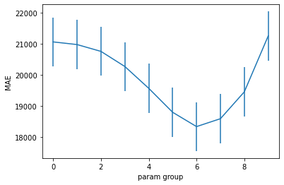
# visualize the search grid
def plot_cv_results(res, confidence=0.95):
    n = len(res['mean_test_score'])
    sem = scipy.stats.sem(res['mean_test_score'])
    t = scipy.stats.t.ppf((1 + confidence) / 2., n-1)
    plt.errorbar(x=range(n), y=-res['mean_test_score'], yerr=t*sem, linetype=None)
    plt.xlabel('param group')
    plt.ylabel('MAE')

plot_cv_results(gs.cv_results_)
gs.best_estimator_
Pipeline(steps=[('preproc',
                 ColumnTransformer(transformers=[('numeric',
                                                  Pipeline(steps=[('fill_na',
                                                                   SimpleImputer(strategy='median')),
                                                                  ('scale',
                                                                   StandardScaler())]),
                                                  ['LotFrontage', 'LotArea',
                                                   'OverallQual', 'OverallCond',
                                                   'YearBuilt', 'YearRemodAdd',
                                                   'MasVnrArea', 'BsmtFinSF1',
                                                   'BsmtFinSF2', 'BsmtUnfSF',
                                                   'TotalBsmtSF', '1stFlrSF',
                                                   '2ndFlrSF', 'LowQualFinSF',
                                                   'GrLivAr...
                                                   'Neighborhood', 'Condition1',
                                                   'Condition2', 'BldgType',
                                                   'HouseStyle', 'RoofStyle',
                                                   'RoofMatl', 'Exterior1st',
                                                   'Exterior2nd', 'MasVnrType',
                                                   'ExterQual', 'ExterCond',
                                                   'Foundation', 'BsmtQual',
                                                   'BsmtCond', 'BsmtExposure',
                                                   'BsmtFinType1',
                                                   'BsmtFinType2', 'Heating',
                                                   'HeatingQC', 'CentralAir',
                                                   'Electrical', ...])],
                                   verbose_feature_names_out=False)),
                ('estimator', Ridge(alpha=21.544346900318846))])
In a Jupyter environment, please rerun this cell to show the HTML representation or trust the notebook. On GitHub, the HTML representation is unable to render, please try loading this page with nbviewer.org.
Pipeline(steps=[('preproc',
                 ColumnTransformer(transformers=[('numeric',
                                                  Pipeline(steps=[('fill_na',
                                                                   SimpleImputer(strategy='median')),
                                                                  ('scale',
                                                                   StandardScaler())]),
                                                  ['LotFrontage', 'LotArea',
                                                   'OverallQual', 'OverallCond',
                                                   'YearBuilt', 'YearRemodAdd',
                                                   'MasVnrArea', 'BsmtFinSF1',
                                                   'BsmtFinSF2', 'BsmtUnfSF',
                                                   'TotalBsmtSF', '1stFlrSF',
                                                   '2ndFlrSF', 'LowQualFinSF',
                                                   'GrLivAr...
                                                   'Neighborhood', 'Condition1',
                                                   'Condition2', 'BldgType',
                                                   'HouseStyle', 'RoofStyle',
                                                   'RoofMatl', 'Exterior1st',
                                                   'Exterior2nd', 'MasVnrType',
                                                   'ExterQual', 'ExterCond',
                                                   'Foundation', 'BsmtQual',
                                                   'BsmtCond', 'BsmtExposure',
                                                   'BsmtFinType1',
                                                   'BsmtFinType2', 'Heating',
                                                   'HeatingQC', 'CentralAir',
                                                   'Electrical', ...])],
                                   verbose_feature_names_out=False)),
('estimator', Ridge(alpha=21.544346900318846))])ColumnTransformer(transformers=[('numeric',
Pipeline(steps=[('fill_na',
SimpleImputer(strategy='median')),
('scale', StandardScaler())]),
['LotFrontage', 'LotArea', 'OverallQual',
'OverallCond', 'YearBuilt', 'YearRemodAdd',
'MasVnrArea', 'BsmtFinSF1', 'BsmtFinSF2',
'BsmtUnfSF', 'TotalBsmtSF', '1stFlrSF',
'2ndFlrSF', 'LowQualFinSF', 'GrLivArea',
'BsmtFullBath', 'BsmtHal...
'LotShape', 'LandContour', 'Utilities',
'LotConfig', 'LandSlope', 'Neighborhood',
'Condition1', 'Condition2', 'BldgType',
'HouseStyle', 'RoofStyle', 'RoofMatl',
'Exterior1st', 'Exterior2nd', 'MasVnrType',
'ExterQual', 'ExterCond', 'Foundation',
'BsmtQual', 'BsmtCond', 'BsmtExposure',
'BsmtFinType1', 'BsmtFinType2', 'Heating',
'HeatingQC', 'CentralAir', 'Electrical', ...])],
verbose_feature_names_out=False)['LotFrontage', 'LotArea', 'OverallQual', 'OverallCond', 'YearBuilt', 'YearRemodAdd', 'MasVnrArea', 'BsmtFinSF1', 'BsmtFinSF2', 'BsmtUnfSF', 'TotalBsmtSF', '1stFlrSF', '2ndFlrSF', 'LowQualFinSF', 'GrLivArea', 'BsmtFullBath', 'BsmtHalfBath', 'FullBath', 'HalfBath', 'BedroomAbvGr', 'KitchenAbvGr', 'TotRmsAbvGrd', 'GarageYrBlt', 'GarageCars', 'GarageArea', 'WoodDeckSF', 'OpenPorchSF', 'EnclosedPorch', '3SsnPorch', 'ScreenPorch', 'PoolArea', 'MiscVal', 'MoSold', 'YrSold']
SimpleImputer(strategy='median')
StandardScaler()
['MSSubClass', 'MSZoning', 'Street', 'LotShape', 'LandContour', 'Utilities', 'LotConfig', 'LandSlope', 'Neighborhood', 'Condition1', 'Condition2', 'BldgType', 'HouseStyle', 'RoofStyle', 'RoofMatl', 'Exterior1st', 'Exterior2nd', 'MasVnrType', 'ExterQual', 'ExterCond', 'Foundation', 'BsmtQual', 'BsmtCond', 'BsmtExposure', 'BsmtFinType1', 'BsmtFinType2', 'Heating', 'HeatingQC', 'CentralAir', 'Electrical', 'KitchenQual', 'Functional', 'Fireplaces', 'FireplaceQu', 'GarageType', 'GarageFinish', 'GarageQual', 'GarageCond', 'PavedDrive', 'Fence', 'SaleType', 'SaleCondition']
SimpleImputer(strategy='most_frequent')
OneHotEncoder(drop='first', handle_unknown='infrequent_if_exist',
min_frequency=5, sparse_output=False)Ridge(alpha=21.544346900318846)
# print stats for each parameter group
def analyze_cv_results(cv_results):
    split_results = np.vstack([val for key, val in cv_results.items() if 'split' in key])

    for ix, p in enumerate(cv_results['params']):
        if ix>0:
            print('-'*30)
        print(f"Parameter group {ix}:", p)
        mu, (lo, hi) = mean_confidence_interval(-split_results[:,ix])
        print(f"\tMean score: {mu:0.2f}")
        print(f"\t95% CI: ({lo:0.2f}, {hi:0.2f})")

analyze_cv_results(gs.cv_results_)
Parameter group 0: {'estimator__alpha': 0.01}
	Mean score: 21054.51
	95% CI: (19528.22, 22580.80)
------------------------------
Parameter group 1: {'estimator__alpha': 0.03593813663804628}
	Mean score: 20969.38
	95% CI: (19455.37, 22483.39)
------------------------------
Parameter group 2: {'estimator__alpha': 0.1291549665014884}
	Mean score: 20749.62
	95% CI: (19260.16, 22239.07)
------------------------------
Parameter group 3: {'estimator__alpha': 0.464158883361278}
	Mean score: 20263.11
	95% CI: (18808.89, 21717.33)
------------------------------
Parameter group 4: {'estimator__alpha': 1.6681005372000592}
	Mean score: 19560.93
	95% CI: (18161.96, 20959.89)
------------------------------
Parameter group 5: {'estimator__alpha': 5.994842503189409}
	Mean score: 18790.41
	95% CI: (17412.15, 20168.66)
------------------------------
Parameter group 6: {'estimator__alpha': 21.544346900318846}
	Mean score: 18330.32
	95% CI: (16920.62, 19740.02)
------------------------------
Parameter group 7: {'estimator__alpha': 77.42636826811278}
	Mean score: 18584.22
	95% CI: (17036.42, 20132.03)
------------------------------
Parameter group 8: {'estimator__alpha': 278.2559402207126}
	Mean score: 19448.43
	95% CI: (18014.46, 20882.41)
------------------------------
Parameter group 9: {'estimator__alpha': 1000.0}
	Mean score: 21247.01
	95% CI: (20167.16, 22326.86)
We get the best mean performance for parameter group 6 with alpha=21.54.
Searching over multiple parameters simultaneously#
Often we will want to search over multiple parameters at the same time. This is easy.
from sklearn.model_selection import GridSearchCV
param_grid = {
    'preproc__numeric__fill_na__strategy': ['mean', 'median', 'most_frequent'],
    'preproc__categorical__encode__min_frequency': [1, 2, 3, 4, 5],
    'estimator__alpha': [21.54]
}
cv = KFold(10, shuffle=True)
gs = GridSearchCV(pipe, param_grid, cv=cv, n_jobs=10, scoring='neg_mean_absolute_error', verbose=True)
gs.fit(X_train, y_train)
gs.best_estimator_
Fitting 10 folds for each of 15 candidates, totalling 150 fits
Pipeline(steps=[('preproc',
                 ColumnTransformer(transformers=[('numeric',
                                                  Pipeline(steps=[('fill_na',
                                                                   SimpleImputer(strategy='most_frequent')),
                                                                  ('scale',
                                                                   StandardScaler())]),
                                                  ['LotFrontage', 'LotArea',
                                                   'OverallQual', 'OverallCond',
                                                   'YearBuilt', 'YearRemodAdd',
                                                   'MasVnrArea', 'BsmtFinSF1',
                                                   'BsmtFinSF2', 'BsmtUnfSF',
                                                   'TotalBsmtSF', '1stFlrSF',
                                                   '2ndFlrSF', 'LowQualFinSF',
                                                   '...
                                                   'Neighborhood', 'Condition1',
                                                   'Condition2', 'BldgType',
                                                   'HouseStyle', 'RoofStyle',
                                                   'RoofMatl', 'Exterior1st',
                                                   'Exterior2nd', 'MasVnrType',
                                                   'ExterQual', 'ExterCond',
                                                   'Foundation', 'BsmtQual',
                                                   'BsmtCond', 'BsmtExposure',
                                                   'BsmtFinType1',
                                                   'BsmtFinType2', 'Heating',
                                                   'HeatingQC', 'CentralAir',
                                                   'Electrical', ...])],
                                   verbose_feature_names_out=False)),
                ('estimator', Ridge(alpha=21.54))])
In a Jupyter environment, please rerun this cell to show the HTML representation or trust the notebook. On GitHub, the HTML representation is unable to render, please try loading this page with nbviewer.org.
Pipeline(steps=[('preproc',
                 ColumnTransformer(transformers=[('numeric',
                                                  Pipeline(steps=[('fill_na',
                                                                   SimpleImputer(strategy='most_frequent')),
                                                                  ('scale',
                                                                   StandardScaler())]),
                                                  ['LotFrontage', 'LotArea',
                                                   'OverallQual', 'OverallCond',
                                                   'YearBuilt', 'YearRemodAdd',
                                                   'MasVnrArea', 'BsmtFinSF1',
                                                   'BsmtFinSF2', 'BsmtUnfSF',
                                                   'TotalBsmtSF', '1stFlrSF',
                                                   '2ndFlrSF', 'LowQualFinSF',
                                                   '...
                                                   'Neighborhood', 'Condition1',
                                                   'Condition2', 'BldgType',
                                                   'HouseStyle', 'RoofStyle',
                                                   'RoofMatl', 'Exterior1st',
                                                   'Exterior2nd', 'MasVnrType',
                                                   'ExterQual', 'ExterCond',
                                                   'Foundation', 'BsmtQual',
                                                   'BsmtCond', 'BsmtExposure',
                                                   'BsmtFinType1',
                                                   'BsmtFinType2', 'Heating',
                                                   'HeatingQC', 'CentralAir',
                                                   'Electrical', ...])],
                                   verbose_feature_names_out=False)),
('estimator', Ridge(alpha=21.54))])ColumnTransformer(transformers=[('numeric',
Pipeline(steps=[('fill_na',
SimpleImputer(strategy='most_frequent')),
('scale', StandardScaler())]),
['LotFrontage', 'LotArea', 'OverallQual',
'OverallCond', 'YearBuilt', 'YearRemodAdd',
'MasVnrArea', 'BsmtFinSF1', 'BsmtFinSF2',
'BsmtUnfSF', 'TotalBsmtSF', '1stFlrSF',
'2ndFlrSF', 'LowQualFinSF', 'GrLivArea',
'BsmtFullBath', '...
'LotShape', 'LandContour', 'Utilities',
'LotConfig', 'LandSlope', 'Neighborhood',
'Condition1', 'Condition2', 'BldgType',
'HouseStyle', 'RoofStyle', 'RoofMatl',
'Exterior1st', 'Exterior2nd', 'MasVnrType',
'ExterQual', 'ExterCond', 'Foundation',
'BsmtQual', 'BsmtCond', 'BsmtExposure',
'BsmtFinType1', 'BsmtFinType2', 'Heating',
'HeatingQC', 'CentralAir', 'Electrical', ...])],
verbose_feature_names_out=False)['LotFrontage', 'LotArea', 'OverallQual', 'OverallCond', 'YearBuilt', 'YearRemodAdd', 'MasVnrArea', 'BsmtFinSF1', 'BsmtFinSF2', 'BsmtUnfSF', 'TotalBsmtSF', '1stFlrSF', '2ndFlrSF', 'LowQualFinSF', 'GrLivArea', 'BsmtFullBath', 'BsmtHalfBath', 'FullBath', 'HalfBath', 'BedroomAbvGr', 'KitchenAbvGr', 'TotRmsAbvGrd', 'GarageYrBlt', 'GarageCars', 'GarageArea', 'WoodDeckSF', 'OpenPorchSF', 'EnclosedPorch', '3SsnPorch', 'ScreenPorch', 'PoolArea', 'MiscVal', 'MoSold', 'YrSold']
SimpleImputer(strategy='most_frequent')
StandardScaler()
['MSSubClass', 'MSZoning', 'Street', 'LotShape', 'LandContour', 'Utilities', 'LotConfig', 'LandSlope', 'Neighborhood', 'Condition1', 'Condition2', 'BldgType', 'HouseStyle', 'RoofStyle', 'RoofMatl', 'Exterior1st', 'Exterior2nd', 'MasVnrType', 'ExterQual', 'ExterCond', 'Foundation', 'BsmtQual', 'BsmtCond', 'BsmtExposure', 'BsmtFinType1', 'BsmtFinType2', 'Heating', 'HeatingQC', 'CentralAir', 'Electrical', 'KitchenQual', 'Functional', 'Fireplaces', 'FireplaceQu', 'GarageType', 'GarageFinish', 'GarageQual', 'GarageCond', 'PavedDrive', 'Fence', 'SaleType', 'SaleCondition']
SimpleImputer(strategy='most_frequent')
OneHotEncoder(drop='first', handle_unknown='infrequent_if_exist',
min_frequency=2, sparse_output=False)Ridge(alpha=21.54)
plot_cv_results(gs.cv_results_)
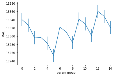
analyze_cv_results(gs.cv_results_)
Parameter group 0: {'estimator__alpha': 21.54, 'preproc__categorical__encode__min_frequency': 1, 'preproc__numeric__fill_na__strategy': 'mean'}
	Mean score: 18340.20
	95% CI: (16399.35, 20281.04)
------------------------------
Parameter group 1: {'estimator__alpha': 21.54, 'preproc__categorical__encode__min_frequency': 1, 'preproc__numeric__fill_na__strategy': 'median'}
	Mean score: 18326.99
	95% CI: (16385.40, 20268.58)
------------------------------
Parameter group 2: {'estimator__alpha': 21.54, 'preproc__categorical__encode__min_frequency': 1, 'preproc__numeric__fill_na__strategy': 'most_frequent'}
	Mean score: 18295.73
	95% CI: (16332.00, 20259.46)
------------------------------
Parameter group 3: {'estimator__alpha': 21.54, 'preproc__categorical__encode__min_frequency': 2, 'preproc__numeric__fill_na__strategy': 'mean'}
	Mean score: 18296.74
	95% CI: (16344.75, 20248.73)
------------------------------
Parameter group 4: {'estimator__alpha': 21.54, 'preproc__categorical__encode__min_frequency': 2, 'preproc__numeric__fill_na__strategy': 'median'}
	Mean score: 18283.10
	95% CI: (16330.26, 20235.94)
------------------------------
Parameter group 5: {'estimator__alpha': 21.54, 'preproc__categorical__encode__min_frequency': 2, 'preproc__numeric__fill_na__strategy': 'most_frequent'}
	Mean score: 18253.03
	95% CI: (16278.90, 20227.17)
------------------------------
Parameter group 6: {'estimator__alpha': 21.54, 'preproc__categorical__encode__min_frequency': 3, 'preproc__numeric__fill_na__strategy': 'mean'}
	Mean score: 18321.84
	95% CI: (16400.77, 20242.91)
------------------------------
Parameter group 7: {'estimator__alpha': 21.54, 'preproc__categorical__encode__min_frequency': 3, 'preproc__numeric__fill_na__strategy': 'median'}
	Mean score: 18310.43
	95% CI: (16388.60, 20232.26)
------------------------------
Parameter group 8: {'estimator__alpha': 21.54, 'preproc__categorical__encode__min_frequency': 3, 'preproc__numeric__fill_na__strategy': 'most_frequent'}
	Mean score: 18284.16
	95% CI: (16345.99, 20222.33)
------------------------------
Parameter group 9: {'estimator__alpha': 21.54, 'preproc__categorical__encode__min_frequency': 4, 'preproc__numeric__fill_na__strategy': 'mean'}
	Mean score: 18341.43
	95% CI: (16408.15, 20274.72)
------------------------------
Parameter group 10: {'estimator__alpha': 21.54, 'preproc__categorical__encode__min_frequency': 4, 'preproc__numeric__fill_na__strategy': 'median'}
	Mean score: 18329.76
	95% CI: (16396.56, 20262.96)
------------------------------
Parameter group 11: {'estimator__alpha': 21.54, 'preproc__categorical__encode__min_frequency': 4, 'preproc__numeric__fill_na__strategy': 'most_frequent'}
	Mean score: 18301.13
	95% CI: (16352.43, 20249.83)
------------------------------
Parameter group 12: {'estimator__alpha': 21.54, 'preproc__categorical__encode__min_frequency': 5, 'preproc__numeric__fill_na__strategy': 'mean'}
	Mean score: 18360.32
	95% CI: (16429.25, 20291.39)
------------------------------
Parameter group 13: {'estimator__alpha': 21.54, 'preproc__categorical__encode__min_frequency': 5, 'preproc__numeric__fill_na__strategy': 'median'}
	Mean score: 18348.10
	95% CI: (16416.62, 20279.58)
------------------------------
Parameter group 14: {'estimator__alpha': 21.54, 'preproc__categorical__encode__min_frequency': 5, 'preproc__numeric__fill_na__strategy': 'most_frequent'}
	Mean score: 18320.57
	95% CI: (16373.19, 20267.95)
It looks like the model prefers ‘most_frequent’ imputation with a OneHotEncoder min frequency of 2.
Searching over different transformers#
Let’s try something a little more drastic. What if we were to replace the imputation approach altogether with a the KNNImputer that we saw earlier in the workshop?
Before, we used GridSearchCV to scan possible values for a parameter in one of our transforms. We can also scan over different transform objects.
pipe
Pipeline(steps=[('preproc',
                 ColumnTransformer(transformers=[('numeric',
                                                  Pipeline(steps=[('fill_na',
                                                                   SimpleImputer(strategy='median')),
                                                                  ('scale',
                                                                   StandardScaler())]),
                                                  ['LotFrontage', 'LotArea',
                                                   'OverallQual', 'OverallCond',
                                                   'YearBuilt', 'YearRemodAdd',
                                                   'MasVnrArea', 'BsmtFinSF1',
                                                   'BsmtFinSF2', 'BsmtUnfSF',
                                                   'TotalBsmtSF', '1stFlrSF',
                                                   '2ndFlrSF', 'LowQualFinSF',
                                                   'GrLivAr...
                                                   'Neighborhood', 'Condition1',
                                                   'Condition2', 'BldgType',
                                                   'HouseStyle', 'RoofStyle',
                                                   'RoofMatl', 'Exterior1st',
                                                   'Exterior2nd', 'MasVnrType',
                                                   'ExterQual', 'ExterCond',
                                                   'Foundation', 'BsmtQual',
                                                   'BsmtCond', 'BsmtExposure',
                                                   'BsmtFinType1',
                                                   'BsmtFinType2', 'Heating',
                                                   'HeatingQC', 'CentralAir',
                                                   'Electrical', ...])],
                                   verbose_feature_names_out=False)),
                ('estimator', Ridge(alpha=1))])
In a Jupyter environment, please rerun this cell to show the HTML representation or trust the notebook. On GitHub, the HTML representation is unable to render, please try loading this page with nbviewer.org.
Pipeline(steps=[('preproc',
                 ColumnTransformer(transformers=[('numeric',
                                                  Pipeline(steps=[('fill_na',
                                                                   SimpleImputer(strategy='median')),
                                                                  ('scale',
                                                                   StandardScaler())]),
                                                  ['LotFrontage', 'LotArea',
                                                   'OverallQual', 'OverallCond',
                                                   'YearBuilt', 'YearRemodAdd',
                                                   'MasVnrArea', 'BsmtFinSF1',
                                                   'BsmtFinSF2', 'BsmtUnfSF',
                                                   'TotalBsmtSF', '1stFlrSF',
                                                   '2ndFlrSF', 'LowQualFinSF',
                                                   'GrLivAr...
                                                   'Neighborhood', 'Condition1',
                                                   'Condition2', 'BldgType',
                                                   'HouseStyle', 'RoofStyle',
                                                   'RoofMatl', 'Exterior1st',
                                                   'Exterior2nd', 'MasVnrType',
                                                   'ExterQual', 'ExterCond',
                                                   'Foundation', 'BsmtQual',
                                                   'BsmtCond', 'BsmtExposure',
                                                   'BsmtFinType1',
                                                   'BsmtFinType2', 'Heating',
                                                   'HeatingQC', 'CentralAir',
                                                   'Electrical', ...])],
                                   verbose_feature_names_out=False)),
('estimator', Ridge(alpha=1))])ColumnTransformer(transformers=[('numeric',
Pipeline(steps=[('fill_na',
SimpleImputer(strategy='median')),
('scale', StandardScaler())]),
['LotFrontage', 'LotArea', 'OverallQual',
'OverallCond', 'YearBuilt', 'YearRemodAdd',
'MasVnrArea', 'BsmtFinSF1', 'BsmtFinSF2',
'BsmtUnfSF', 'TotalBsmtSF', '1stFlrSF',
'2ndFlrSF', 'LowQualFinSF', 'GrLivArea',
'BsmtFullBath', 'BsmtHal...
'LotShape', 'LandContour', 'Utilities',
'LotConfig', 'LandSlope', 'Neighborhood',
'Condition1', 'Condition2', 'BldgType',
'HouseStyle', 'RoofStyle', 'RoofMatl',
'Exterior1st', 'Exterior2nd', 'MasVnrType',
'ExterQual', 'ExterCond', 'Foundation',
'BsmtQual', 'BsmtCond', 'BsmtExposure',
'BsmtFinType1', 'BsmtFinType2', 'Heating',
'HeatingQC', 'CentralAir', 'Electrical', ...])],
verbose_feature_names_out=False)['LotFrontage', 'LotArea', 'OverallQual', 'OverallCond', 'YearBuilt', 'YearRemodAdd', 'MasVnrArea', 'BsmtFinSF1', 'BsmtFinSF2', 'BsmtUnfSF', 'TotalBsmtSF', '1stFlrSF', '2ndFlrSF', 'LowQualFinSF', 'GrLivArea', 'BsmtFullBath', 'BsmtHalfBath', 'FullBath', 'HalfBath', 'BedroomAbvGr', 'KitchenAbvGr', 'TotRmsAbvGrd', 'GarageYrBlt', 'GarageCars', 'GarageArea', 'WoodDeckSF', 'OpenPorchSF', 'EnclosedPorch', '3SsnPorch', 'ScreenPorch', 'PoolArea', 'MiscVal', 'MoSold', 'YrSold']
SimpleImputer(strategy='median')
StandardScaler()
['MSSubClass', 'MSZoning', 'Street', 'LotShape', 'LandContour', 'Utilities', 'LotConfig', 'LandSlope', 'Neighborhood', 'Condition1', 'Condition2', 'BldgType', 'HouseStyle', 'RoofStyle', 'RoofMatl', 'Exterior1st', 'Exterior2nd', 'MasVnrType', 'ExterQual', 'ExterCond', 'Foundation', 'BsmtQual', 'BsmtCond', 'BsmtExposure', 'BsmtFinType1', 'BsmtFinType2', 'Heating', 'HeatingQC', 'CentralAir', 'Electrical', 'KitchenQual', 'Functional', 'Fireplaces', 'FireplaceQu', 'GarageType', 'GarageFinish', 'GarageQual', 'GarageCond', 'PavedDrive', 'Fence', 'SaleType', 'SaleCondition']
SimpleImputer(strategy='most_frequent')
OneHotEncoder(drop='first', handle_unknown='infrequent_if_exist',
min_frequency=5, sparse_output=False)Ridge(alpha=1)
from sklearn.impute import KNNImputer
param_grid = {
    # before: 'preproc__numeric__fill_na__strategy': ['mean', 'median', 'most_frequent'],
    'preproc__numeric__fill_na': [SimpleImputer(strategy='most_frequent'), KNNImputer(n_neighbors=20, weights="uniform")],
    'preproc__categorical__encode__min_frequency': [2],
    'estimator__alpha': [21.54]
}

gs = GridSearchCV(pipe, param_grid, cv=cv, n_jobs=10, scoring='neg_mean_absolute_error', verbose=True)
gs.fit(X_train, y_train)
gs.best_estimator_
Fitting 10 folds for each of 2 candidates, totalling 20 fits
Pipeline(steps=[('preproc',
                 ColumnTransformer(transformers=[('numeric',
                                                  Pipeline(steps=[('fill_na',
                                                                   SimpleImputer(strategy='most_frequent')),
                                                                  ('scale',
                                                                   StandardScaler())]),
                                                  ['LotFrontage', 'LotArea',
                                                   'OverallQual', 'OverallCond',
                                                   'YearBuilt', 'YearRemodAdd',
                                                   'MasVnrArea', 'BsmtFinSF1',
                                                   'BsmtFinSF2', 'BsmtUnfSF',
                                                   'TotalBsmtSF', '1stFlrSF',
                                                   '2ndFlrSF', 'LowQualFinSF',
                                                   '...
                                                   'Neighborhood', 'Condition1',
                                                   'Condition2', 'BldgType',
                                                   'HouseStyle', 'RoofStyle',
                                                   'RoofMatl', 'Exterior1st',
                                                   'Exterior2nd', 'MasVnrType',
                                                   'ExterQual', 'ExterCond',
                                                   'Foundation', 'BsmtQual',
                                                   'BsmtCond', 'BsmtExposure',
                                                   'BsmtFinType1',
                                                   'BsmtFinType2', 'Heating',
                                                   'HeatingQC', 'CentralAir',
                                                   'Electrical', ...])],
                                   verbose_feature_names_out=False)),
                ('estimator', Ridge(alpha=21.54))])
In a Jupyter environment, please rerun this cell to show the HTML representation or trust the notebook. On GitHub, the HTML representation is unable to render, please try loading this page with nbviewer.org.
Pipeline(steps=[('preproc',
                 ColumnTransformer(transformers=[('numeric',
                                                  Pipeline(steps=[('fill_na',
                                                                   SimpleImputer(strategy='most_frequent')),
                                                                  ('scale',
                                                                   StandardScaler())]),
                                                  ['LotFrontage', 'LotArea',
                                                   'OverallQual', 'OverallCond',
                                                   'YearBuilt', 'YearRemodAdd',
                                                   'MasVnrArea', 'BsmtFinSF1',
                                                   'BsmtFinSF2', 'BsmtUnfSF',
                                                   'TotalBsmtSF', '1stFlrSF',
                                                   '2ndFlrSF', 'LowQualFinSF',
                                                   '...
                                                   'Neighborhood', 'Condition1',
                                                   'Condition2', 'BldgType',
                                                   'HouseStyle', 'RoofStyle',
                                                   'RoofMatl', 'Exterior1st',
                                                   'Exterior2nd', 'MasVnrType',
                                                   'ExterQual', 'ExterCond',
                                                   'Foundation', 'BsmtQual',
                                                   'BsmtCond', 'BsmtExposure',
                                                   'BsmtFinType1',
                                                   'BsmtFinType2', 'Heating',
                                                   'HeatingQC', 'CentralAir',
                                                   'Electrical', ...])],
                                   verbose_feature_names_out=False)),
('estimator', Ridge(alpha=21.54))])ColumnTransformer(transformers=[('numeric',
Pipeline(steps=[('fill_na',
SimpleImputer(strategy='most_frequent')),
('scale', StandardScaler())]),
['LotFrontage', 'LotArea', 'OverallQual',
'OverallCond', 'YearBuilt', 'YearRemodAdd',
'MasVnrArea', 'BsmtFinSF1', 'BsmtFinSF2',
'BsmtUnfSF', 'TotalBsmtSF', '1stFlrSF',
'2ndFlrSF', 'LowQualFinSF', 'GrLivArea',
'BsmtFullBath', '...
'LotShape', 'LandContour', 'Utilities',
'LotConfig', 'LandSlope', 'Neighborhood',
'Condition1', 'Condition2', 'BldgType',
'HouseStyle', 'RoofStyle', 'RoofMatl',
'Exterior1st', 'Exterior2nd', 'MasVnrType',
'ExterQual', 'ExterCond', 'Foundation',
'BsmtQual', 'BsmtCond', 'BsmtExposure',
'BsmtFinType1', 'BsmtFinType2', 'Heating',
'HeatingQC', 'CentralAir', 'Electrical', ...])],
verbose_feature_names_out=False)['LotFrontage', 'LotArea', 'OverallQual', 'OverallCond', 'YearBuilt', 'YearRemodAdd', 'MasVnrArea', 'BsmtFinSF1', 'BsmtFinSF2', 'BsmtUnfSF', 'TotalBsmtSF', '1stFlrSF', '2ndFlrSF', 'LowQualFinSF', 'GrLivArea', 'BsmtFullBath', 'BsmtHalfBath', 'FullBath', 'HalfBath', 'BedroomAbvGr', 'KitchenAbvGr', 'TotRmsAbvGrd', 'GarageYrBlt', 'GarageCars', 'GarageArea', 'WoodDeckSF', 'OpenPorchSF', 'EnclosedPorch', '3SsnPorch', 'ScreenPorch', 'PoolArea', 'MiscVal', 'MoSold', 'YrSold']
SimpleImputer(strategy='most_frequent')
StandardScaler()
['MSSubClass', 'MSZoning', 'Street', 'LotShape', 'LandContour', 'Utilities', 'LotConfig', 'LandSlope', 'Neighborhood', 'Condition1', 'Condition2', 'BldgType', 'HouseStyle', 'RoofStyle', 'RoofMatl', 'Exterior1st', 'Exterior2nd', 'MasVnrType', 'ExterQual', 'ExterCond', 'Foundation', 'BsmtQual', 'BsmtCond', 'BsmtExposure', 'BsmtFinType1', 'BsmtFinType2', 'Heating', 'HeatingQC', 'CentralAir', 'Electrical', 'KitchenQual', 'Functional', 'Fireplaces', 'FireplaceQu', 'GarageType', 'GarageFinish', 'GarageQual', 'GarageCond', 'PavedDrive', 'Fence', 'SaleType', 'SaleCondition']
SimpleImputer(strategy='most_frequent')
OneHotEncoder(drop='first', handle_unknown='infrequent_if_exist',
min_frequency=2, sparse_output=False)Ridge(alpha=21.54)
plot_cv_results(gs.cv_results_)
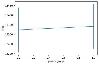
analyze_cv_results(gs.cv_results_)
Parameter group 0: {'estimator__alpha': 21.54, 'preproc__categorical__encode__min_frequency': 2, 'preproc__numeric__fill_na': SimpleImputer(strategy='most_frequent')}
	Mean score: 18322.53
	95% CI: (15369.93, 21275.13)
------------------------------
Parameter group 1: {'estimator__alpha': 21.54, 'preproc__categorical__encode__min_frequency': 2, 'preproc__numeric__fill_na': KNNImputer(n_neighbors=20)}
	Mean score: 18340.86
	95% CI: (15379.45, 21302.27)
We can’t distinguish between these two approaches.
Searching different estimators#
Just like we could search over different transforms, we can search over different estimators.
from sklearn.ensemble import RandomForestRegressor, GradientBoostingRegressor

param_grid = {
    'preproc__numeric__fill_na': [SimpleImputer(strategy='most_frequent')],
    'preproc__categorical__encode__min_frequency': [2],
    'estimator': [Ridge(alpha=21.54), RandomForestRegressor(), GradientBoostingRegressor()]
}

gs = GridSearchCV(pipe, param_grid, cv=cv, n_jobs=10, scoring='neg_mean_absolute_error', verbose=True)
gs.fit(X_train, y_train)
gs.best_estimator_
Fitting 10 folds for each of 3 candidates, totalling 30 fits
Pipeline(steps=[('preproc',
                 ColumnTransformer(transformers=[('numeric',
                                                  Pipeline(steps=[('fill_na',
                                                                   SimpleImputer(strategy='most_frequent')),
                                                                  ('scale',
                                                                   StandardScaler())]),
                                                  ['LotFrontage', 'LotArea',
                                                   'OverallQual', 'OverallCond',
                                                   'YearBuilt', 'YearRemodAdd',
                                                   'MasVnrArea', 'BsmtFinSF1',
                                                   'BsmtFinSF2', 'BsmtUnfSF',
                                                   'TotalBsmtSF', '1stFlrSF',
                                                   '2ndFlrSF', 'LowQualFinSF',
                                                   '...
                                                   'Neighborhood', 'Condition1',
                                                   'Condition2', 'BldgType',
                                                   'HouseStyle', 'RoofStyle',
                                                   'RoofMatl', 'Exterior1st',
                                                   'Exterior2nd', 'MasVnrType',
                                                   'ExterQual', 'ExterCond',
                                                   'Foundation', 'BsmtQual',
                                                   'BsmtCond', 'BsmtExposure',
                                                   'BsmtFinType1',
                                                   'BsmtFinType2', 'Heating',
                                                   'HeatingQC', 'CentralAir',
                                                   'Electrical', ...])],
                                   verbose_feature_names_out=False)),
                ('estimator', GradientBoostingRegressor())])
In a Jupyter environment, please rerun this cell to show the HTML representation or trust the notebook. On GitHub, the HTML representation is unable to render, please try loading this page with nbviewer.org.
Pipeline(steps=[('preproc',
                 ColumnTransformer(transformers=[('numeric',
                                                  Pipeline(steps=[('fill_na',
                                                                   SimpleImputer(strategy='most_frequent')),
                                                                  ('scale',
                                                                   StandardScaler())]),
                                                  ['LotFrontage', 'LotArea',
                                                   'OverallQual', 'OverallCond',
                                                   'YearBuilt', 'YearRemodAdd',
                                                   'MasVnrArea', 'BsmtFinSF1',
                                                   'BsmtFinSF2', 'BsmtUnfSF',
                                                   'TotalBsmtSF', '1stFlrSF',
                                                   '2ndFlrSF', 'LowQualFinSF',
                                                   '...
                                                   'Neighborhood', 'Condition1',
                                                   'Condition2', 'BldgType',
                                                   'HouseStyle', 'RoofStyle',
                                                   'RoofMatl', 'Exterior1st',
                                                   'Exterior2nd', 'MasVnrType',
                                                   'ExterQual', 'ExterCond',
                                                   'Foundation', 'BsmtQual',
                                                   'BsmtCond', 'BsmtExposure',
                                                   'BsmtFinType1',
                                                   'BsmtFinType2', 'Heating',
                                                   'HeatingQC', 'CentralAir',
                                                   'Electrical', ...])],
                                   verbose_feature_names_out=False)),
('estimator', GradientBoostingRegressor())])ColumnTransformer(transformers=[('numeric',
Pipeline(steps=[('fill_na',
SimpleImputer(strategy='most_frequent')),
('scale', StandardScaler())]),
['LotFrontage', 'LotArea', 'OverallQual',
'OverallCond', 'YearBuilt', 'YearRemodAdd',
'MasVnrArea', 'BsmtFinSF1', 'BsmtFinSF2',
'BsmtUnfSF', 'TotalBsmtSF', '1stFlrSF',
'2ndFlrSF', 'LowQualFinSF', 'GrLivArea',
'BsmtFullBath', '...
'LotShape', 'LandContour', 'Utilities',
'LotConfig', 'LandSlope', 'Neighborhood',
'Condition1', 'Condition2', 'BldgType',
'HouseStyle', 'RoofStyle', 'RoofMatl',
'Exterior1st', 'Exterior2nd', 'MasVnrType',
'ExterQual', 'ExterCond', 'Foundation',
'BsmtQual', 'BsmtCond', 'BsmtExposure',
'BsmtFinType1', 'BsmtFinType2', 'Heating',
'HeatingQC', 'CentralAir', 'Electrical', ...])],
verbose_feature_names_out=False)['LotFrontage', 'LotArea', 'OverallQual', 'OverallCond', 'YearBuilt', 'YearRemodAdd', 'MasVnrArea', 'BsmtFinSF1', 'BsmtFinSF2', 'BsmtUnfSF', 'TotalBsmtSF', '1stFlrSF', '2ndFlrSF', 'LowQualFinSF', 'GrLivArea', 'BsmtFullBath', 'BsmtHalfBath', 'FullBath', 'HalfBath', 'BedroomAbvGr', 'KitchenAbvGr', 'TotRmsAbvGrd', 'GarageYrBlt', 'GarageCars', 'GarageArea', 'WoodDeckSF', 'OpenPorchSF', 'EnclosedPorch', '3SsnPorch', 'ScreenPorch', 'PoolArea', 'MiscVal', 'MoSold', 'YrSold']
SimpleImputer(strategy='most_frequent')
StandardScaler()
['MSSubClass', 'MSZoning', 'Street', 'LotShape', 'LandContour', 'Utilities', 'LotConfig', 'LandSlope', 'Neighborhood', 'Condition1', 'Condition2', 'BldgType', 'HouseStyle', 'RoofStyle', 'RoofMatl', 'Exterior1st', 'Exterior2nd', 'MasVnrType', 'ExterQual', 'ExterCond', 'Foundation', 'BsmtQual', 'BsmtCond', 'BsmtExposure', 'BsmtFinType1', 'BsmtFinType2', 'Heating', 'HeatingQC', 'CentralAir', 'Electrical', 'KitchenQual', 'Functional', 'Fireplaces', 'FireplaceQu', 'GarageType', 'GarageFinish', 'GarageQual', 'GarageCond', 'PavedDrive', 'Fence', 'SaleType', 'SaleCondition']
SimpleImputer(strategy='most_frequent')
OneHotEncoder(drop='first', handle_unknown='infrequent_if_exist',
min_frequency=2, sparse_output=False)GradientBoostingRegressor()
plot_cv_results(gs.cv_results_)
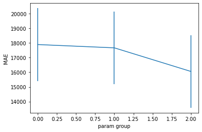
analyze_cv_results(gs.cv_results_)
Parameter group 0: {'estimator': Ridge(alpha=21.54), 'preproc__categorical__encode__min_frequency': 2, 'preproc__numeric__fill_na': SimpleImputer(strategy='most_frequent')}
	Mean score: 17885.12
	95% CI: (16272.11, 19498.13)
------------------------------
Parameter group 1: {'estimator': RandomForestRegressor(), 'preproc__categorical__encode__min_frequency': 2, 'preproc__numeric__fill_na': SimpleImputer(strategy='most_frequent')}
	Mean score: 17662.02
	95% CI: (16542.67, 18781.37)
------------------------------
Parameter group 2: {'estimator': GradientBoostingRegressor(), 'preproc__categorical__encode__min_frequency': 2, 'preproc__numeric__fill_na': SimpleImputer(strategy='most_frequent')}
	Mean score: 16056.59
	95% CI: (15043.17, 17070.01)
Random Forest and Gradient boosting might have an edge, but there’s a lot of overlap in the CIs. At this point, one might want to focus on tuning the hyperparameters for the tree-based models.
For now, though, let’s see how to implement dimension reduction in our pipeline.
Dimension reduction#
We can insert a PCA step into our pipeline.
from sklearn.decomposition import PCA

pipe = Pipeline([
    ('preproc', preproc),
    ('feature_selection', PCA(n_components=10)),
    ('estimator', Ridge(alpha=1))
])

pipe
Pipeline(steps=[('preproc',
                 ColumnTransformer(transformers=[('numeric',
                                                  Pipeline(steps=[('fill_na',
                                                                   SimpleImputer(strategy='median')),
                                                                  ('scale',
                                                                   StandardScaler())]),
                                                  ['LotFrontage', 'LotArea',
                                                   'OverallQual', 'OverallCond',
                                                   'YearBuilt', 'YearRemodAdd',
                                                   'MasVnrArea', 'BsmtFinSF1',
                                                   'BsmtFinSF2', 'BsmtUnfSF',
                                                   'TotalBsmtSF', '1stFlrSF',
                                                   '2ndFlrSF', 'LowQualFinSF',
                                                   'GrLivAr...
                                                   'Condition2', 'BldgType',
                                                   'HouseStyle', 'RoofStyle',
                                                   'RoofMatl', 'Exterior1st',
                                                   'Exterior2nd', 'MasVnrType',
                                                   'ExterQual', 'ExterCond',
                                                   'Foundation', 'BsmtQual',
                                                   'BsmtCond', 'BsmtExposure',
                                                   'BsmtFinType1',
                                                   'BsmtFinType2', 'Heating',
                                                   'HeatingQC', 'CentralAir',
                                                   'Electrical', ...])],
                                   verbose_feature_names_out=False)),
                ('feature_selection', PCA(n_components=10)),
                ('estimator', Ridge(alpha=1))])
In a Jupyter environment, please rerun this cell to show the HTML representation or trust the notebook. On GitHub, the HTML representation is unable to render, please try loading this page with nbviewer.org.
Pipeline(steps=[('preproc',
                 ColumnTransformer(transformers=[('numeric',
                                                  Pipeline(steps=[('fill_na',
                                                                   SimpleImputer(strategy='median')),
                                                                  ('scale',
                                                                   StandardScaler())]),
                                                  ['LotFrontage', 'LotArea',
                                                   'OverallQual', 'OverallCond',
                                                   'YearBuilt', 'YearRemodAdd',
                                                   'MasVnrArea', 'BsmtFinSF1',
                                                   'BsmtFinSF2', 'BsmtUnfSF',
                                                   'TotalBsmtSF', '1stFlrSF',
                                                   '2ndFlrSF', 'LowQualFinSF',
                                                   'GrLivAr...
                                                   'Condition2', 'BldgType',
                                                   'HouseStyle', 'RoofStyle',
                                                   'RoofMatl', 'Exterior1st',
                                                   'Exterior2nd', 'MasVnrType',
                                                   'ExterQual', 'ExterCond',
                                                   'Foundation', 'BsmtQual',
                                                   'BsmtCond', 'BsmtExposure',
                                                   'BsmtFinType1',
                                                   'BsmtFinType2', 'Heating',
                                                   'HeatingQC', 'CentralAir',
                                                   'Electrical', ...])],
                                   verbose_feature_names_out=False)),
                ('feature_selection', PCA(n_components=10)),
('estimator', Ridge(alpha=1))])ColumnTransformer(transformers=[('numeric',
Pipeline(steps=[('fill_na',
SimpleImputer(strategy='median')),
('scale', StandardScaler())]),
['LotFrontage', 'LotArea', 'OverallQual',
'OverallCond', 'YearBuilt', 'YearRemodAdd',
'MasVnrArea', 'BsmtFinSF1', 'BsmtFinSF2',
'BsmtUnfSF', 'TotalBsmtSF', '1stFlrSF',
'2ndFlrSF', 'LowQualFinSF', 'GrLivArea',
'BsmtFullBath', 'BsmtHal...
'LotShape', 'LandContour', 'Utilities',
'LotConfig', 'LandSlope', 'Neighborhood',
'Condition1', 'Condition2', 'BldgType',
'HouseStyle', 'RoofStyle', 'RoofMatl',
'Exterior1st', 'Exterior2nd', 'MasVnrType',
'ExterQual', 'ExterCond', 'Foundation',
'BsmtQual', 'BsmtCond', 'BsmtExposure',
'BsmtFinType1', 'BsmtFinType2', 'Heating',
'HeatingQC', 'CentralAir', 'Electrical', ...])],
verbose_feature_names_out=False)['LotFrontage', 'LotArea', 'OverallQual', 'OverallCond', 'YearBuilt', 'YearRemodAdd', 'MasVnrArea', 'BsmtFinSF1', 'BsmtFinSF2', 'BsmtUnfSF', 'TotalBsmtSF', '1stFlrSF', '2ndFlrSF', 'LowQualFinSF', 'GrLivArea', 'BsmtFullBath', 'BsmtHalfBath', 'FullBath', 'HalfBath', 'BedroomAbvGr', 'KitchenAbvGr', 'TotRmsAbvGrd', 'GarageYrBlt', 'GarageCars', 'GarageArea', 'WoodDeckSF', 'OpenPorchSF', 'EnclosedPorch', '3SsnPorch', 'ScreenPorch', 'PoolArea', 'MiscVal', 'MoSold', 'YrSold']
SimpleImputer(strategy='median')
StandardScaler()
['MSSubClass', 'MSZoning', 'Street', 'LotShape', 'LandContour', 'Utilities', 'LotConfig', 'LandSlope', 'Neighborhood', 'Condition1', 'Condition2', 'BldgType', 'HouseStyle', 'RoofStyle', 'RoofMatl', 'Exterior1st', 'Exterior2nd', 'MasVnrType', 'ExterQual', 'ExterCond', 'Foundation', 'BsmtQual', 'BsmtCond', 'BsmtExposure', 'BsmtFinType1', 'BsmtFinType2', 'Heating', 'HeatingQC', 'CentralAir', 'Electrical', 'KitchenQual', 'Functional', 'Fireplaces', 'FireplaceQu', 'GarageType', 'GarageFinish', 'GarageQual', 'GarageCond', 'PavedDrive', 'Fence', 'SaleType', 'SaleCondition']
SimpleImputer(strategy='most_frequent')
OneHotEncoder(drop='first', handle_unknown='infrequent_if_exist',
min_frequency=5, sparse_output=False)PCA(n_components=10)
Ridge(alpha=1)
# now lets fit new pipeline and see how it does
# we add a "passthrough" to the parameter search
param_grid = {
    'preproc__numeric__fill_na': [SimpleImputer(strategy='most_frequent')],
    'preproc__categorical__encode__min_frequency': [2],
    'feature_selection': ["passthrough"] + [PCA(n) for n in range(1,100,10)],
    'estimator__alpha': [21.54]
}

gs = GridSearchCV(pipe, param_grid, cv=cv, n_jobs=10, scoring='neg_mean_absolute_error', verbose=True)
gs.fit(X_train, y_train)
gs.best_estimator_
Fitting 10 folds for each of 11 candidates, totalling 110 fits
Pipeline(steps=[('preproc',
                 ColumnTransformer(transformers=[('numeric',
                                                  Pipeline(steps=[('fill_na',
                                                                   SimpleImputer(strategy='most_frequent')),
                                                                  ('scale',
                                                                   StandardScaler())]),
                                                  ['LotFrontage', 'LotArea',
                                                   'OverallQual', 'OverallCond',
                                                   'YearBuilt', 'YearRemodAdd',
                                                   'MasVnrArea', 'BsmtFinSF1',
                                                   'BsmtFinSF2', 'BsmtUnfSF',
                                                   'TotalBsmtSF', '1stFlrSF',
                                                   '2ndFlrSF', 'LowQualFinSF',
                                                   '...
                                                   'Condition2', 'BldgType',
                                                   'HouseStyle', 'RoofStyle',
                                                   'RoofMatl', 'Exterior1st',
                                                   'Exterior2nd', 'MasVnrType',
                                                   'ExterQual', 'ExterCond',
                                                   'Foundation', 'BsmtQual',
                                                   'BsmtCond', 'BsmtExposure',
                                                   'BsmtFinType1',
                                                   'BsmtFinType2', 'Heating',
                                                   'HeatingQC', 'CentralAir',
                                                   'Electrical', ...])],
                                   verbose_feature_names_out=False)),
                ('feature_selection', 'passthrough'),
                ('estimator', Ridge(alpha=21.54))])
In a Jupyter environment, please rerun this cell to show the HTML representation or trust the notebook. On GitHub, the HTML representation is unable to render, please try loading this page with nbviewer.org.
Pipeline(steps=[('preproc',
                 ColumnTransformer(transformers=[('numeric',
                                                  Pipeline(steps=[('fill_na',
                                                                   SimpleImputer(strategy='most_frequent')),
                                                                  ('scale',
                                                                   StandardScaler())]),
                                                  ['LotFrontage', 'LotArea',
                                                   'OverallQual', 'OverallCond',
                                                   'YearBuilt', 'YearRemodAdd',
                                                   'MasVnrArea', 'BsmtFinSF1',
                                                   'BsmtFinSF2', 'BsmtUnfSF',
                                                   'TotalBsmtSF', '1stFlrSF',
                                                   '2ndFlrSF', 'LowQualFinSF',
                                                   '...
                                                   'Condition2', 'BldgType',
                                                   'HouseStyle', 'RoofStyle',
                                                   'RoofMatl', 'Exterior1st',
                                                   'Exterior2nd', 'MasVnrType',
                                                   'ExterQual', 'ExterCond',
                                                   'Foundation', 'BsmtQual',
                                                   'BsmtCond', 'BsmtExposure',
                                                   'BsmtFinType1',
                                                   'BsmtFinType2', 'Heating',
                                                   'HeatingQC', 'CentralAir',
                                                   'Electrical', ...])],
                                   verbose_feature_names_out=False)),
                ('feature_selection', 'passthrough'),
('estimator', Ridge(alpha=21.54))])ColumnTransformer(transformers=[('numeric',
Pipeline(steps=[('fill_na',
SimpleImputer(strategy='most_frequent')),
('scale', StandardScaler())]),
['LotFrontage', 'LotArea', 'OverallQual',
'OverallCond', 'YearBuilt', 'YearRemodAdd',
'MasVnrArea', 'BsmtFinSF1', 'BsmtFinSF2',
'BsmtUnfSF', 'TotalBsmtSF', '1stFlrSF',
'2ndFlrSF', 'LowQualFinSF', 'GrLivArea',
'BsmtFullBath', '...
'LotShape', 'LandContour', 'Utilities',
'LotConfig', 'LandSlope', 'Neighborhood',
'Condition1', 'Condition2', 'BldgType',
'HouseStyle', 'RoofStyle', 'RoofMatl',
'Exterior1st', 'Exterior2nd', 'MasVnrType',
'ExterQual', 'ExterCond', 'Foundation',
'BsmtQual', 'BsmtCond', 'BsmtExposure',
'BsmtFinType1', 'BsmtFinType2', 'Heating',
'HeatingQC', 'CentralAir', 'Electrical', ...])],
verbose_feature_names_out=False)['LotFrontage', 'LotArea', 'OverallQual', 'OverallCond', 'YearBuilt', 'YearRemodAdd', 'MasVnrArea', 'BsmtFinSF1', 'BsmtFinSF2', 'BsmtUnfSF', 'TotalBsmtSF', '1stFlrSF', '2ndFlrSF', 'LowQualFinSF', 'GrLivArea', 'BsmtFullBath', 'BsmtHalfBath', 'FullBath', 'HalfBath', 'BedroomAbvGr', 'KitchenAbvGr', 'TotRmsAbvGrd', 'GarageYrBlt', 'GarageCars', 'GarageArea', 'WoodDeckSF', 'OpenPorchSF', 'EnclosedPorch', '3SsnPorch', 'ScreenPorch', 'PoolArea', 'MiscVal', 'MoSold', 'YrSold']
SimpleImputer(strategy='most_frequent')
StandardScaler()
['MSSubClass', 'MSZoning', 'Street', 'LotShape', 'LandContour', 'Utilities', 'LotConfig', 'LandSlope', 'Neighborhood', 'Condition1', 'Condition2', 'BldgType', 'HouseStyle', 'RoofStyle', 'RoofMatl', 'Exterior1st', 'Exterior2nd', 'MasVnrType', 'ExterQual', 'ExterCond', 'Foundation', 'BsmtQual', 'BsmtCond', 'BsmtExposure', 'BsmtFinType1', 'BsmtFinType2', 'Heating', 'HeatingQC', 'CentralAir', 'Electrical', 'KitchenQual', 'Functional', 'Fireplaces', 'FireplaceQu', 'GarageType', 'GarageFinish', 'GarageQual', 'GarageCond', 'PavedDrive', 'Fence', 'SaleType', 'SaleCondition']
SimpleImputer(strategy='most_frequent')
OneHotEncoder(drop='first', handle_unknown='infrequent_if_exist',
              min_frequency=2, sparse_output=False)
passthrough
Ridge(alpha=21.54)
plot_cv_results(gs.cv_results_)
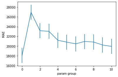
The passthrough variant outperforms all of the PCA variants. Let’s try a different feature selection approach.
from sklearn.feature_selection import SelectKBest
from sklearn.feature_selection import f_classif
# now lets fit new pipeline and see how it does
# we add a "passthrough" to the parameter search
param_grid = {
    'preproc__numeric__fill_na': [SimpleImputer(strategy='most_frequent')],
    'preproc__categorical__encode__min_frequency': [2],
    'feature_selection': ["passthrough"] + [SelectKBest(f_classif, k=k) for k in range(1, 200, 40)],
    'estimator__alpha': [21.54]
}

gs = GridSearchCV(pipe, param_grid, cv=cv, n_jobs=10, scoring='neg_mean_absolute_error', verbose=True)
gs.fit(X_train, y_train)
gs.best_estimator_
Fitting 10 folds for each of 6 candidates, totalling 60 fits
Pipeline(steps=[('preproc',
                 ColumnTransformer(transformers=[('numeric',
                                                  Pipeline(steps=[('fill_na',
                                                                   SimpleImputer(strategy='most_frequent')),
                                                                  ('scale',
                                                                   StandardScaler())]),
                                                  ['LotFrontage', 'LotArea',
                                                   'OverallQual', 'OverallCond',
                                                   'YearBuilt', 'YearRemodAdd',
                                                   'MasVnrArea', 'BsmtFinSF1',
                                                   'BsmtFinSF2', 'BsmtUnfSF',
                                                   'TotalBsmtSF', '1stFlrSF',
                                                   '2ndFlrSF', 'LowQualFinSF',
                                                   '...
                                                   'Condition2', 'BldgType',
                                                   'HouseStyle', 'RoofStyle',
                                                   'RoofMatl', 'Exterior1st',
                                                   'Exterior2nd', 'MasVnrType',
                                                   'ExterQual', 'ExterCond',
                                                   'Foundation', 'BsmtQual',
                                                   'BsmtCond', 'BsmtExposure',
                                                   'BsmtFinType1',
                                                   'BsmtFinType2', 'Heating',
                                                   'HeatingQC', 'CentralAir',
                                                   'Electrical', ...])],
                                   verbose_feature_names_out=False)),
                ('feature_selection', 'passthrough'),
                ('estimator', Ridge(alpha=21.54))])
In a Jupyter environment, please rerun this cell to show the HTML representation or trust the notebook. On GitHub, the HTML representation is unable to render, please try loading this page with nbviewer.org.
Pipeline(steps=[('preproc',
                 ColumnTransformer(transformers=[('numeric',
                                                  Pipeline(steps=[('fill_na',
                                                                   SimpleImputer(strategy='most_frequent')),
                                                                  ('scale',
                                                                   StandardScaler())]),
                                                  ['LotFrontage', 'LotArea',
                                                   'OverallQual', 'OverallCond',
                                                   'YearBuilt', 'YearRemodAdd',
                                                   'MasVnrArea', 'BsmtFinSF1',
                                                   'BsmtFinSF2', 'BsmtUnfSF',
                                                   'TotalBsmtSF', '1stFlrSF',
                                                   '2ndFlrSF', 'LowQualFinSF',
                                                   '...
                                                   'Condition2', 'BldgType',
                                                   'HouseStyle', 'RoofStyle',
                                                   'RoofMatl', 'Exterior1st',
                                                   'Exterior2nd', 'MasVnrType',
                                                   'ExterQual', 'ExterCond',
                                                   'Foundation', 'BsmtQual',
                                                   'BsmtCond', 'BsmtExposure',
                                                   'BsmtFinType1',
                                                   'BsmtFinType2', 'Heating',
                                                   'HeatingQC', 'CentralAir',
                                                   'Electrical', ...])],
                                   verbose_feature_names_out=False)),
                ('feature_selection', 'passthrough'),
('estimator', Ridge(alpha=21.54))])ColumnTransformer(transformers=[('numeric',
Pipeline(steps=[('fill_na',
SimpleImputer(strategy='most_frequent')),
('scale', StandardScaler())]),
['LotFrontage', 'LotArea', 'OverallQual',
'OverallCond', 'YearBuilt', 'YearRemodAdd',
'MasVnrArea', 'BsmtFinSF1', 'BsmtFinSF2',
'BsmtUnfSF', 'TotalBsmtSF', '1stFlrSF',
'2ndFlrSF', 'LowQualFinSF', 'GrLivArea',
'BsmtFullBath', '...
'LotShape', 'LandContour', 'Utilities',
'LotConfig', 'LandSlope', 'Neighborhood',
'Condition1', 'Condition2', 'BldgType',
'HouseStyle', 'RoofStyle', 'RoofMatl',
'Exterior1st', 'Exterior2nd', 'MasVnrType',
'ExterQual', 'ExterCond', 'Foundation',
'BsmtQual', 'BsmtCond', 'BsmtExposure',
'BsmtFinType1', 'BsmtFinType2', 'Heating',
'HeatingQC', 'CentralAir', 'Electrical', ...])],
verbose_feature_names_out=False)['LotFrontage', 'LotArea', 'OverallQual', 'OverallCond', 'YearBuilt', 'YearRemodAdd', 'MasVnrArea', 'BsmtFinSF1', 'BsmtFinSF2', 'BsmtUnfSF', 'TotalBsmtSF', '1stFlrSF', '2ndFlrSF', 'LowQualFinSF', 'GrLivArea', 'BsmtFullBath', 'BsmtHalfBath', 'FullBath', 'HalfBath', 'BedroomAbvGr', 'KitchenAbvGr', 'TotRmsAbvGrd', 'GarageYrBlt', 'GarageCars', 'GarageArea', 'WoodDeckSF', 'OpenPorchSF', 'EnclosedPorch', '3SsnPorch', 'ScreenPorch', 'PoolArea', 'MiscVal', 'MoSold', 'YrSold']
SimpleImputer(strategy='most_frequent')
StandardScaler()
['MSSubClass', 'MSZoning', 'Street', 'LotShape', 'LandContour', 'Utilities', 'LotConfig', 'LandSlope', 'Neighborhood', 'Condition1', 'Condition2', 'BldgType', 'HouseStyle', 'RoofStyle', 'RoofMatl', 'Exterior1st', 'Exterior2nd', 'MasVnrType', 'ExterQual', 'ExterCond', 'Foundation', 'BsmtQual', 'BsmtCond', 'BsmtExposure', 'BsmtFinType1', 'BsmtFinType2', 'Heating', 'HeatingQC', 'CentralAir', 'Electrical', 'KitchenQual', 'Functional', 'Fireplaces', 'FireplaceQu', 'GarageType', 'GarageFinish', 'GarageQual', 'GarageCond', 'PavedDrive', 'Fence', 'SaleType', 'SaleCondition']
SimpleImputer(strategy='most_frequent')
OneHotEncoder(drop='first', handle_unknown='infrequent_if_exist',
              min_frequency=2, sparse_output=False)
passthrough
Ridge(alpha=21.54)
plot_cv_results(gs.cv_results_)
analyze_cv_results(gs.cv_results_)
Parameter group 0: {'estimator__alpha': 21.54, 'feature_selection': 'passthrough', 'preproc__categorical__encode__min_frequency': 2, 'preproc__numeric__fill_na': SimpleImputer(strategy='most_frequent')}
	Mean score: 18313.82
	95% CI: (15610.21, 21017.43)
------------------------------
Parameter group 1: {'estimator__alpha': 21.54, 'feature_selection': SelectKBest(k=1), 'preproc__categorical__encode__min_frequency': 2, 'preproc__numeric__fill_na': SimpleImputer(strategy='most_frequent')}
	Mean score: 56349.52
	95% CI: (52760.24, 59938.79)
------------------------------
Parameter group 2: {'estimator__alpha': 21.54, 'feature_selection': SelectKBest(k=41), 'preproc__categorical__encode__min_frequency': 2, 'preproc__numeric__fill_na': SimpleImputer(strategy='most_frequent')}
	Mean score: 21874.57
	95% CI: (19566.05, 24183.08)
------------------------------
Parameter group 3: {'estimator__alpha': 21.54, 'feature_selection': SelectKBest(k=81), 'preproc__categorical__encode__min_frequency': 2, 'preproc__numeric__fill_na': SimpleImputer(strategy='most_frequent')}
	Mean score: 19809.51
	95% CI: (17204.10, 22414.92)
------------------------------
Parameter group 4: {'estimator__alpha': 21.54, 'feature_selection': SelectKBest(k=121), 'preproc__categorical__encode__min_frequency': 2, 'preproc__numeric__fill_na': SimpleImputer(strategy='most_frequent')}
	Mean score: 19531.81
	95% CI: (17051.55, 22012.07)
------------------------------
Parameter group 5: {'estimator__alpha': 21.54, 'feature_selection': SelectKBest(k=161), 'preproc__categorical__encode__min_frequency': 2, 'preproc__numeric__fill_na': SimpleImputer(strategy='most_frequent')}
	Mean score: 19106.24
	95% CI: (16654.09, 21558.40)
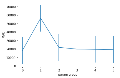
“passthrough” wins again, though we retain most of the performance using only 41 features.
Final Evaluation#
We can view the best estimator from the search and evaluate it on the test set. This estimator was selected using cross validation then retrained on the entire train set.
gs.best_estimator_
Pipeline(steps=[('preproc',
                 ColumnTransformer(transformers=[('numeric',
                                                  Pipeline(steps=[('fill_na',
                                                                   SimpleImputer(strategy='most_frequent')),
                                                                  ('scale',
                                                                   StandardScaler())]),
                                                  ['LotFrontage', 'LotArea',
                                                   'OverallQual', 'OverallCond',
                                                   'YearBuilt', 'YearRemodAdd',
                                                   'MasVnrArea', 'BsmtFinSF1',
                                                   'BsmtFinSF2', 'BsmtUnfSF',
                                                   'TotalBsmtSF', '1stFlrSF',
                                                   '2ndFlrSF', 'LowQualFinSF',
                                                   '...
                                                   'Condition2', 'BldgType',
                                                   'HouseStyle', 'RoofStyle',
                                                   'RoofMatl', 'Exterior1st',
                                                   'Exterior2nd', 'MasVnrType',
                                                   'ExterQual', 'ExterCond',
                                                   'Foundation', 'BsmtQual',
                                                   'BsmtCond', 'BsmtExposure',
                                                   'BsmtFinType1',
                                                   'BsmtFinType2', 'Heating',
                                                   'HeatingQC', 'CentralAir',
                                                   'Electrical', ...])],
                                   verbose_feature_names_out=False)),
                ('feature_selection', 'passthrough'),
                ('estimator', Ridge(alpha=21.54))])
In a Jupyter environment, please rerun this cell to show the HTML representation or trust the notebook. On GitHub, the HTML representation is unable to render, please try loading this page with nbviewer.org.
Pipeline(steps=[('preproc',
                 ColumnTransformer(transformers=[('numeric',
                                                  Pipeline(steps=[('fill_na',
                                                                   SimpleImputer(strategy='most_frequent')),
                                                                  ('scale',
                                                                   StandardScaler())]),
                                                  ['LotFrontage', 'LotArea',
                                                   'OverallQual', 'OverallCond',
                                                   'YearBuilt', 'YearRemodAdd',
                                                   'MasVnrArea', 'BsmtFinSF1',
                                                   'BsmtFinSF2', 'BsmtUnfSF',
                                                   'TotalBsmtSF', '1stFlrSF',
                                                   '2ndFlrSF', 'LowQualFinSF',
                                                   '...
                                                   'Condition2', 'BldgType',
                                                   'HouseStyle', 'RoofStyle',
                                                   'RoofMatl', 'Exterior1st',
                                                   'Exterior2nd', 'MasVnrType',
                                                   'ExterQual', 'ExterCond',
                                                   'Foundation', 'BsmtQual',
                                                   'BsmtCond', 'BsmtExposure',
                                                   'BsmtFinType1',
                                                   'BsmtFinType2', 'Heating',
                                                   'HeatingQC', 'CentralAir',
                                                   'Electrical', ...])],
                                   verbose_feature_names_out=False)),
                ('feature_selection', 'passthrough'),
('estimator', Ridge(alpha=21.54))])ColumnTransformer(transformers=[('numeric',
Pipeline(steps=[('fill_na',
SimpleImputer(strategy='most_frequent')),
('scale', StandardScaler())]),
['LotFrontage', 'LotArea', 'OverallQual',
'OverallCond', 'YearBuilt', 'YearRemodAdd',
'MasVnrArea', 'BsmtFinSF1', 'BsmtFinSF2',
'BsmtUnfSF', 'TotalBsmtSF', '1stFlrSF',
'2ndFlrSF', 'LowQualFinSF', 'GrLivArea',
'BsmtFullBath', '...
'LotShape', 'LandContour', 'Utilities',
'LotConfig', 'LandSlope', 'Neighborhood',
'Condition1', 'Condition2', 'BldgType',
'HouseStyle', 'RoofStyle', 'RoofMatl',
'Exterior1st', 'Exterior2nd', 'MasVnrType',
'ExterQual', 'ExterCond', 'Foundation',
'BsmtQual', 'BsmtCond', 'BsmtExposure',
'BsmtFinType1', 'BsmtFinType2', 'Heating',
'HeatingQC', 'CentralAir', 'Electrical', ...])],
verbose_feature_names_out=False)['LotFrontage', 'LotArea', 'OverallQual', 'OverallCond', 'YearBuilt', 'YearRemodAdd', 'MasVnrArea', 'BsmtFinSF1', 'BsmtFinSF2', 'BsmtUnfSF', 'TotalBsmtSF', '1stFlrSF', '2ndFlrSF', 'LowQualFinSF', 'GrLivArea', 'BsmtFullBath', 'BsmtHalfBath', 'FullBath', 'HalfBath', 'BedroomAbvGr', 'KitchenAbvGr', 'TotRmsAbvGrd', 'GarageYrBlt', 'GarageCars', 'GarageArea', 'WoodDeckSF', 'OpenPorchSF', 'EnclosedPorch', '3SsnPorch', 'ScreenPorch', 'PoolArea', 'MiscVal', 'MoSold', 'YrSold']
SimpleImputer(strategy='most_frequent')
StandardScaler()
['MSSubClass', 'MSZoning', 'Street', 'LotShape', 'LandContour', 'Utilities', 'LotConfig', 'LandSlope', 'Neighborhood', 'Condition1', 'Condition2', 'BldgType', 'HouseStyle', 'RoofStyle', 'RoofMatl', 'Exterior1st', 'Exterior2nd', 'MasVnrType', 'ExterQual', 'ExterCond', 'Foundation', 'BsmtQual', 'BsmtCond', 'BsmtExposure', 'BsmtFinType1', 'BsmtFinType2', 'Heating', 'HeatingQC', 'CentralAir', 'Electrical', 'KitchenQual', 'Functional', 'Fireplaces', 'FireplaceQu', 'GarageType', 'GarageFinish', 'GarageQual', 'GarageCond', 'PavedDrive', 'Fence', 'SaleType', 'SaleCondition']
SimpleImputer(strategy='most_frequent')
OneHotEncoder(drop='first', handle_unknown='infrequent_if_exist',
              min_frequency=2, sparse_output=False)
passthrough
Ridge(alpha=21.54)
# MAE is a more intuitive metric for price estimation
from sklearn.metrics import mean_absolute_error, r2_score

print("First-pass performance:")
print("Train MAE:", mean_absolute_error(y_train, y_train_pred_1stpass))
print("Test MAE:", mean_absolute_error(y_test, y_test_pred_1stpass))
print("Train R^2:", r2_score(y_train, y_train_pred_1stpass))
print("Test R^2:", r2_score(y_test, y_test_pred_1stpass))

y_train_pred = gs.best_estimator_.predict(X_train)
y_test_pred = gs.best_estimator_.predict(X_test)
print("\nFine tuned performance:")
print("Train MAE:", mean_absolute_error(y_train, y_train_pred))
print("Test MAE:", mean_absolute_error(y_test, y_test_pred))
print("Train R^2:", r2_score(y_train, y_train_pred))
print("Test R^2:", r2_score(y_test, y_test_pred))
First-pass performance:
Train MAE: 15288.339516024189
Test MAE: 20544.401602914677
Train R^2: 0.9028881797596011
Test R^2: 0.8714648323729995

Fine tuned performance:
Train MAE: 15485.129766251588
Test MAE: 18672.381852407823
Train R^2: 0.8875868898505703
Test R^2: 0.8765177538936448
Assignment#
If you didn’t already, apply the methodology described above to your own dataset. Explore additional ways to improve the model. For instance, we saw that GradientBoostingRegressor had an edge on Ridge regression without any hyperparameter tuning. Explore the hyperparameters for GradientBoostingRegressor on the sklearn documentation page. Define a hyperparameter search using GridSearchCV and use our evaluation methodology to compare the two methods.